


Originally presented as a live talk on November 5, 2025

Background
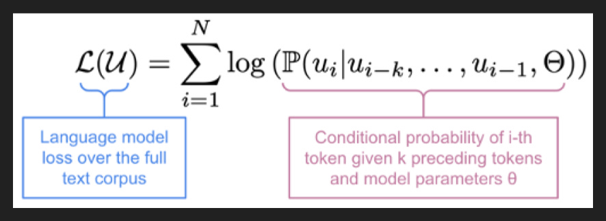
So to really understand this paper, we have to understand loss.
“Loss” is what ML folks call the mismatch between what you wanted the model to do and what the model actually did. A perfect model would always have zero loss, and a terrible model will have really high loss. More loss means we need to make bigger changes to the model to get somewhere good.
To measure this loss, we use a loss function. Here’s the loss function for pretraining actually. It says the loss for each token to predict is just the log of that token’s probability when it comes time to predict that token. If the model is perfect and the probability is 1, then log of 1 is 0, so the loss is zero. If the model is terrible and the probability is close to zero, log of zero is a very large number, so your loss can be huge. Technically the loss would be a very large negative number, but people like dealing with positive numbers so usually you’ll see a little negative sign tacked on to this.
So if you’re training on a big pretraining corpus of like 30T tokens, you’re going to get the loss for each of those tokens and then sum it all up. And that’s what you’re trying to minimize in pretraining.
This is also the loss we use in SFT! We don’t count the user tokens in the loss function since the model doesn’t predict those, but otherwise it’s exactly the same. And this loss function is why SFT is like imitation and can lead to memorization and why it’s great for enforcing formatting and so on, because the SFT loss is lowest when the model produces the exact token that was in the training data. Even synonyms will incur a loss; predicting “amazing” when the training data says “wonderful” still hurts. Very inflexible but sometimes that’s what you’re after.
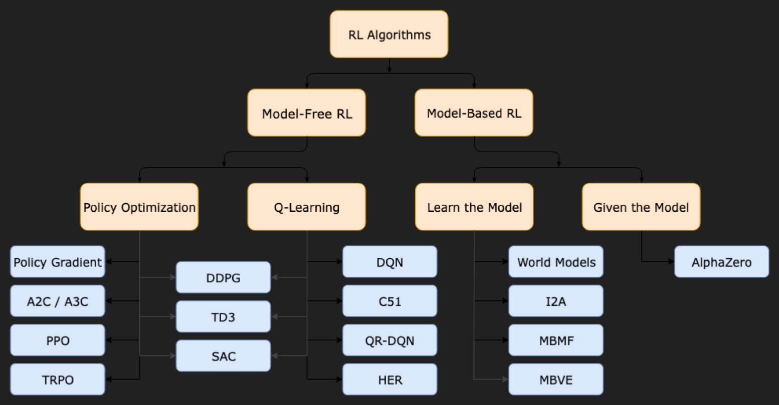
For RL things get a little bit… messier. That’s because there are many different algorithms for RL.
Let’s review: in reinforcement learning, you give rewards for certain outcomes. For RLVR, you give a reward for a verifiable answer, like the answer to a math problem or the confirmation email when a computer use agent makes a purchase. For Rubrics, you give a reward for each satisfied criterion. For RLHF, you give a reward when your reward model picks the right response in a preference rank. Simple enough, but where does this reward information actually go?
That’s where all these different RL algorithms come in. REINFORCE, PPO, GRPO, and all the other versions are just ways of turning rewards into losses.
This here is a rough and incomplete taxonomy of RL algorithms. Even if you’re familiar with RL training for LLMs, you probably have never heard of most of these. In fact the only one on here you typically will see is PPO, Proximal Policy Optimization.
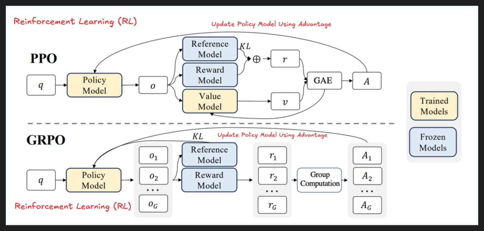
And actually within PPO are many variants: REINFORCE, RLOO, CISPO and so on. The most famous version is GRPO, Group Relative Policy Optimization.
Briefly, PPO requires this thing called a “value model” to say how valuable each token in a response is. You compare that value to the reward you got for your entire response - whether from a rule like in RLVR or from a reward model like in RLHF - and the difference between the overall reward and the value at that token says how valuable the next predicted token ended up being.
So on the image above, a prompt q gets a response o. That response gets a reward, in this case from a reward model but could be rule-based like in RLVR. You also see how far away you are from your reference model, so you don’t stray too far from a known good model. That’s called KL divergence, hence the KL in the diagram. Anyway the reward and the KL divergence together produce r. You also get the value v of each token in the response with that value model. You compare r and v using this formula called “generalized advantage estimation”, and that finally produces the advantage A. You need all that stuff for your loss function.
GRPO simplifies PPO by getting rid of the value model. Instead, you give the same credit to all tokens in your response. But now you need something like the value function that provides a baseline, a way to say “this is normal” vs “this is better and should be encouraged” or “this is worse and should be discouraged”. GRPO does this by normalizing the rewards, basically taking the average of all your responses to a prompt and seeing which ones are relatively the best.
So in the image above, you get multiple responses, each one gets a reward, and you normalize them to get an advantage for each response.
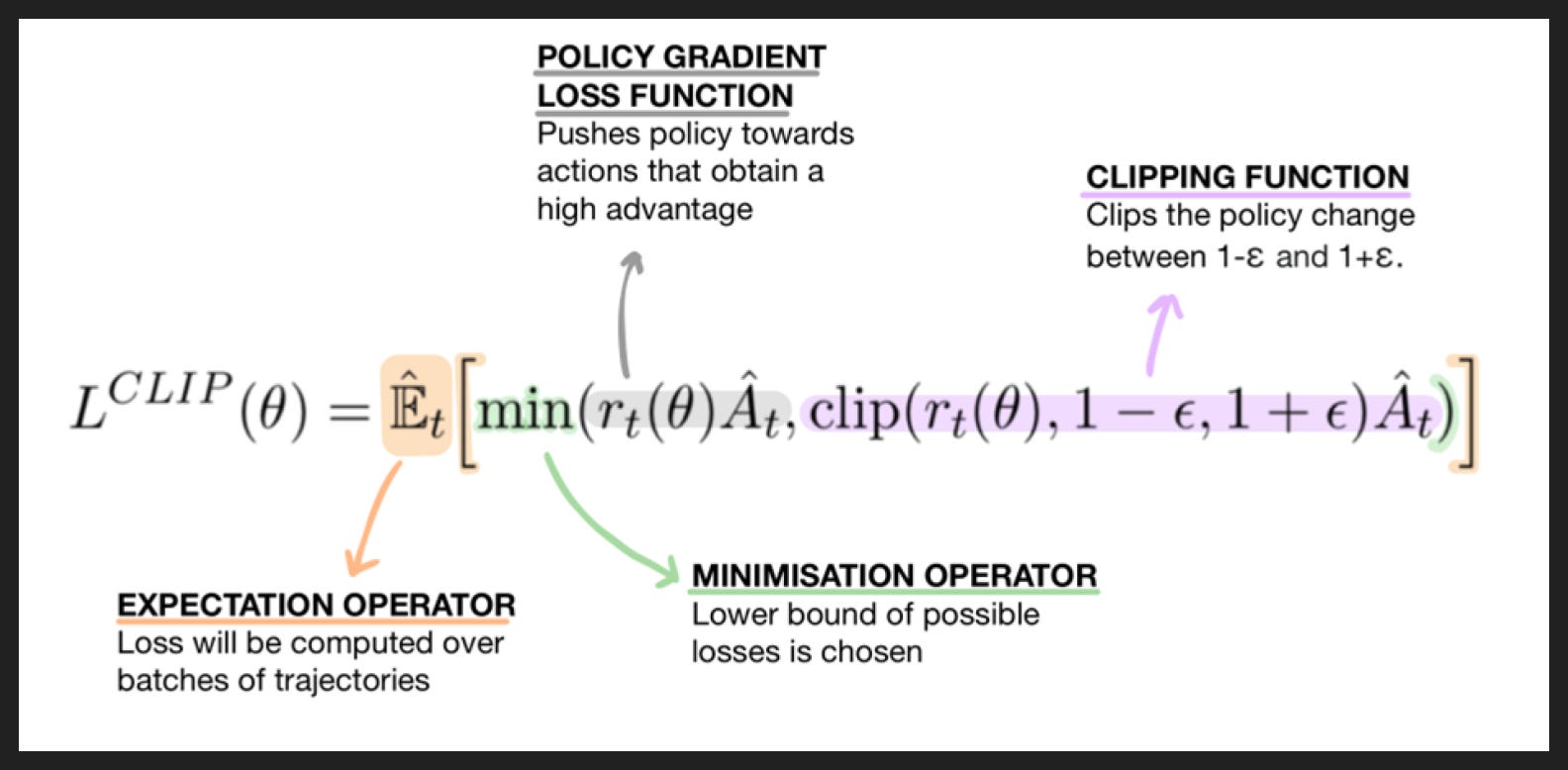
Here’s a simple version of that PPO loss function. We see our friend the advantage A, and also r which compares the current model with the reference model. The CLIP part basically says we only want to make changes up to a certain amount, even if some of our signals say we should make really big changes. The 1 - epsilon and 1 + epsilon parts control how big that maximum change is.
The main ingredient here is that advantage A, which depends on the reward and also the value where applicable. So from a data perspective, accurate rewards are the only thing we can influence. If we make an RLVR problem with the wrong answer or a rubric with missing criteria, the loss function isn’t going to point us in the right direction of how to change our model in training.
Compare all this to SFT, where yes, each token in the response we write influences the loss function, but also how much simpler the SFT loss function is. RL has way more knobs to fiddle.
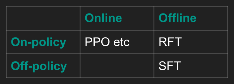
Finally I want to clarify two pairs of terms I often see confused.
One is on-policy vs off-policy. This is just a fancy way of saying “the data came from this model” or “the data came from somewhere else”. So for example SFT, which usually comes from a human writing the ideal response to a prompt, is off-policy. But the RL we’re familiar with, like RLHF where we get two responses from a model or RLVR where we get a response from a model then grade it, that’s gonna be on-policy.
RFT, which stands for “rejection-sampling fine-tuning”, is when you generate responses from the model you want to train and keep only the good ones, based on whatever criteria you have, and then do supervised fine-tuning on them. That’s on-policy, but it’s offline; those good examples go into your dataset and stay there, like they’re still good responses no matter what later happens to your model.
Online means you don’t keep your data after training, you regenerate after you train. The RLHF we’re used to is like this, where we need to generate new data when there’s a new version of the model to train.
Usually online and on-policy go together, which is why you hear them conflated. Same with offline and off-policy. But they are distinct.
The Paper
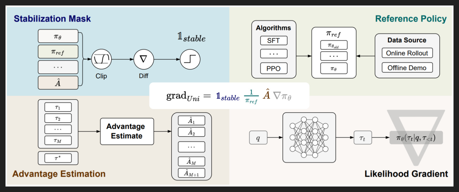
So with all that background, we are at least somewhat equipped to understand their main theoretical point: that SFT and many RL techniques can be viewed as different versions of the same loss function, written here in the middle. Technically their “unified policy gradient estimator” here is the negative of the loss, but all the lessons we draw will be the same.
Anyway, we have four components:
The likelihood gradient - this means the action we’ll take is ultimately to adjust the model weights
The advantage estimate - this says we adjust more based on how good the response was
The reference policy - this is where you say whether you’re comparing to an older version of your model or not
The stabilization mask - this is for clipping
Not every algorithm has every one of these, but you can put in dummy values or terms that cancel each other out to make this universal form work. The helpful part is how it pulls out each of these four universal ingredients.
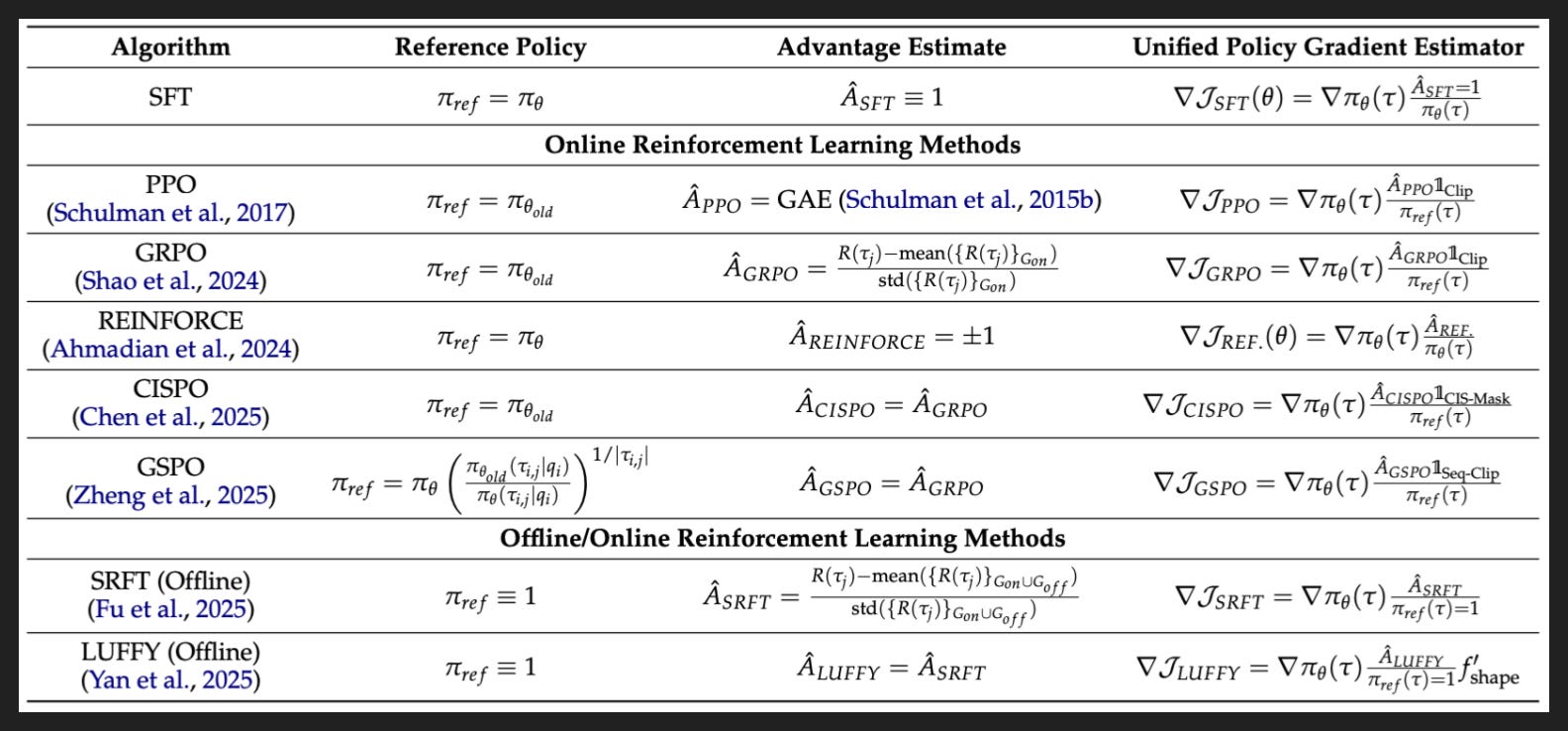
Here is how they translate various algorithms into their framework. Let me touch on the algorithms first and then explain the translation.
SFT, PPO, and GRPO we already know. REINFORCE is actually an ancestor of PPO from before the era of LLMs, but the 2024 paper they attach to it here is applying REINFORCE to LLMs - either way it’s basically PPO but without the value function. CISPO and GSPO are offshoots of GRPO.
SRFT and LUFFY are not important to distinguish individually, but you’ll see they’re grouped under “Offline/Online RL Methods”. They are direct competitors to the method the authors of this paper are going to reveal, so we’ll wait until then to discuss what this title really means.
Now the reference policy is what the algorithm compares to when seeing how big of an update to make. If a correct token is predicted to be highly likely by the reference model, make a small update. If a correct token is predicted to be highly unlikely by the reference model, make a big update. Pi-zero here means the current model, pi-zero-old means an older but still recent version of the model. Using the most recent version is higher risk but higher reward; if you’ve been training and your current version is untested because you just finished one cycle of training, you don’t actually know if it’s better or worse than the last version you tested.
That’s why some algorithms use an older, fixed version that they have tested. Your updates are going to be anchored to your fixed reference model here, which means less risk but also less reward, since your fixed reference model may actually be quite far away from the global optimum.
Don’t worry about the GSPO one, it’s too complicated to get into here.
Okay, next is advantage estimate. We talked about PPO and GRPO in detail. For SFT the advantage of every token is 1 because in SFT every token of the response in the training data is supposed to be the ideal token. Again, that’s why SFT is like imitation or memorization. REINFORCE is actually similar, but you get -1 across the board for a bad response.
And when you put everything together in the right column, you can see that the gradient is indeed a function of these four components. There was no column for the stabilization mask but it’s in the final formula, like you can see 1-CLIP in PPO and GRPO.
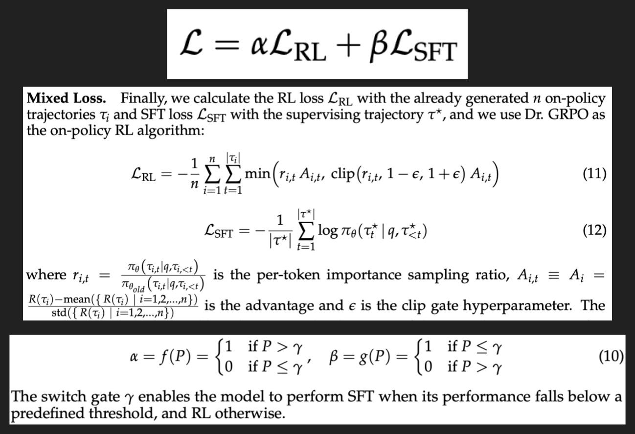
So what is their practical innovation here? Well it’s to do with those two algorithms from the last slide that I didn’t explain, under “Offline/Online RL Methods”.
The idea is much more simple than all this fancy language makes it seem: if SFT and RL have different strengths, can you do better by mixing them? Or another way of looking at it: instead of choosing a certain amount of SFT to do and then a certain amount of RL to do afterwards, what if we discovered the right mix during training?
The top formula there encapsulates it: let’s make the loss a combination, a weighted sum of the SFT loss and the RL loss.
The second screenshot there shows the exact loss formulas they used in their experiments, but you could use a different RL loss from a different algorithm if you wanted to. Theirs is a variant of GRPO called Dr. GRPO. Hopefully you have a rough idea what this is saying by now - look at the relative likelihoods of a token for the current vs reference model, see how advantageous it was, do that for all your tokens across all your different responses to the same prompt, that’s your loss.
The third screenshot is the definitions of alpha and beta, the coefficients that determine how much of each loss goes into your final loss. The math looks fancy, but really all it’s saying is that if your model gets at least some threshold of correct responses to a prompt, where gamma is that threshold, then just use the RL loss function. If your model doesn’t hit that threshold, just use the SFT loss function. It doesn’t actually recommend a mix of both on any one problem at any one time - alpha and beta are binary, and when one of them is on the other is off. The mix that you discover is when to switch loss functions per problem, per training step.
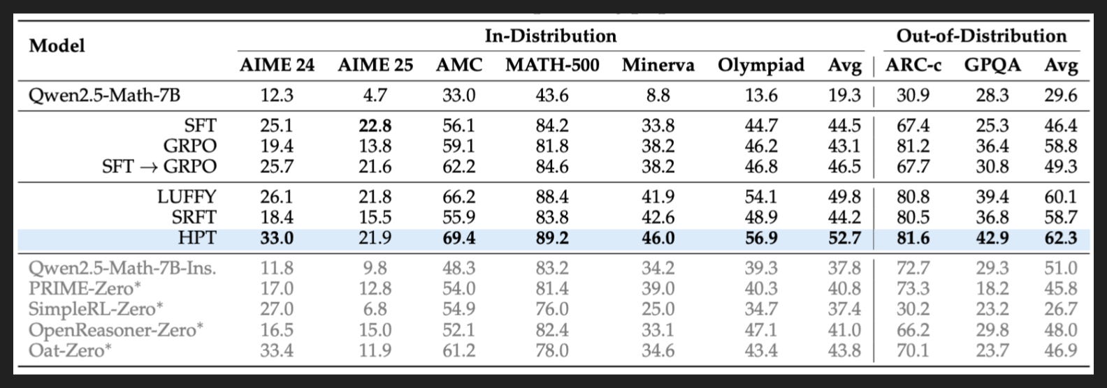
So does this work? And how much better is it?
Well they train a couple models, mostly Qwen2.5-Math-7B, on a bunch of math benchmarks. The rows show the base model, then just SFT, then just GRPO, then SFT followed by GRPO, which are all standard patterns. Unsurprisingly, SFT followed by RL does the best, as is traditional.
The next section down is three different hybrid techniques, including theirs, Hybrid Post-Training or HPT. HPT does better than all the other techniques on all benchmarks except for one, including on the two benchmarks they didn’t specifically train for as shown on the right.
The other entries in grey we don’t need to worry about, they’re just other attempts at math post-training on the same base model. That comparison is less instructive but good to see how HPT stacks up with other respected techniques.

Now one charge they need to defend against is something called the Elicitation Hypothesis.
The Elicitation Hypothesis asserts that RLVR, using whatever algorithm you want, doesn’t actually teach the model anything new; instead, it makes hidden knowledge or abilities come to the fore, it elicits rather than teaching. So your RLVR’d model gets more things right on the first or maybe second or third attempt only because it has prioritized a correct solution that it otherwise would rarely produce.
The way that some papers have shown the Elicitation Hypothesis to be true is with charts like this, where you take a really high number of samples from your model and see if any of them have a correct solution in them. In the jargon, that would be pass@k for very large k, like 1024 in this case. If your base model hits the same pass@ large k that your RLVR’d model does, that means the base model had the solution in there the whole time and that RLVR just elicited it. So what you’d see on a chart like this is two lines, with one line starting above the other but then the two lines meeting at a big enough k.
But that’s not what you see on these charts, at least not totally. In the first chart that’s not what you see at all actually - the lines for HPT and Base Model are basically parallel, so it seems like the model really learned something new from HPT.
The second chart is more mixed, with performance leveling off for HPT while it still goes up for Base Model. So perhaps HPT is doing some elicitation but also some teaching, and we’re hitting the limit of this small model’s performance at 85% or so.
The third chart is the most Elicitation-like, although the model is getting basically 100% so there’s really nowhere else to go. Still, if the base model can get nearly 100% without any training if you just give it enough chances, then maybe HPT only could elicit, since apparently almost all the answers were in there somewhere.
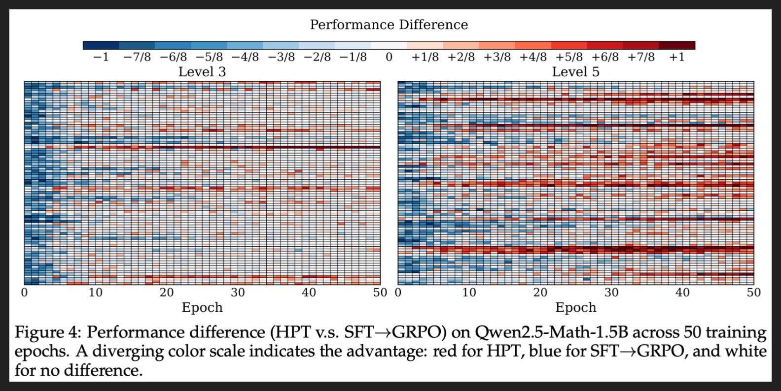
Now this is a fun one. It’s showing how HPT stacks up against the traditional SFT then RL combo on the exact same set of problems. Each row is a problem from the dataset, and Level 3 and Level 5 are two different difficulty levels of problems. Blue means SFT then RL did a better job, red means HPT did a better job. The denominator on the key is 8 because at each step they’re generating 8 responses to the problem and grading each one.
So as you train more, as you go through more epochs of training, the chart generally shifts from blue to red, or at least to white which means no difference. In some cases it’s a pretty dark red, meaning HPT got the model to get 8/8 attempts right but SFT then RL made the model get 8/8 attempts wrong.
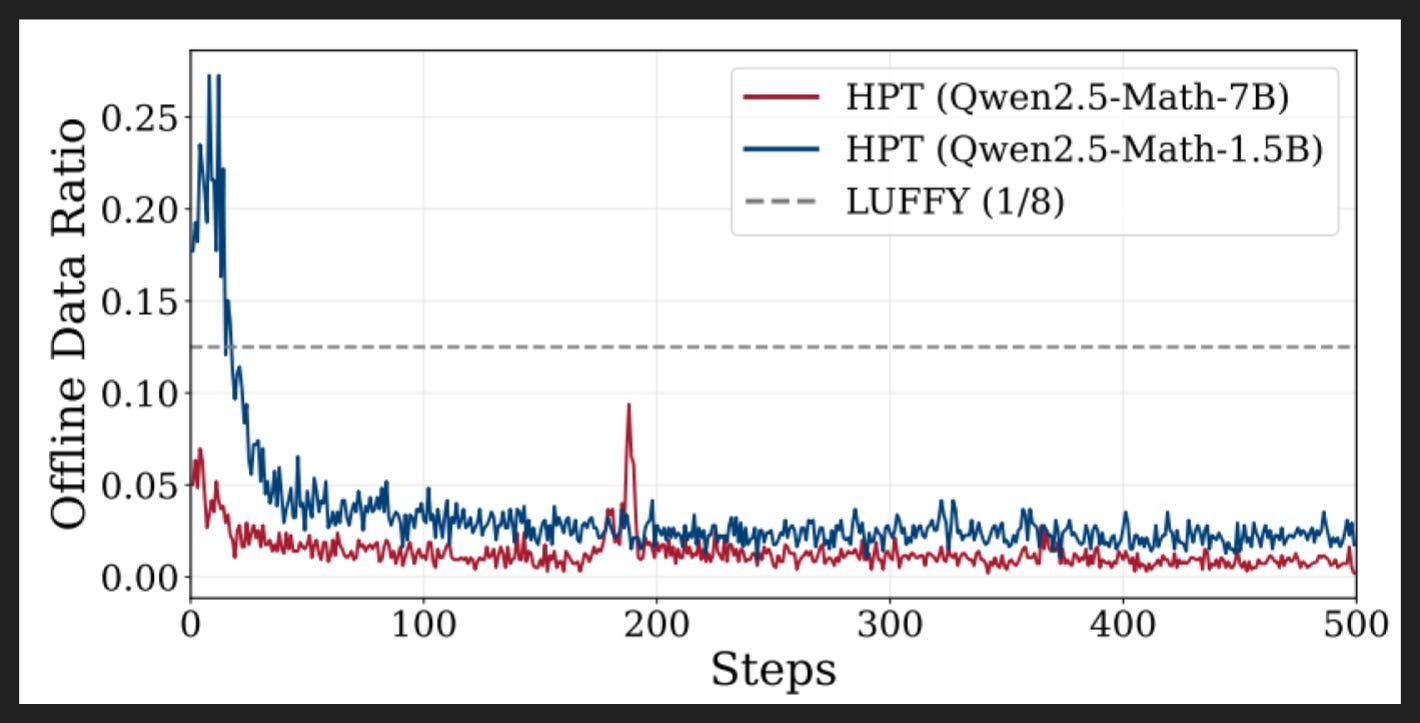
Here’s a quick look at the mix of SFT and RL. The higher the number, the higher the ratio of problems that used SFT, which in this case happened when the model got all 8 of its attempts wrong.
The weaker model needs more SFT the whole time, especially in the beginning, but in both cases it’s a small share most of the time. But apparently that small share makes a significant difference!
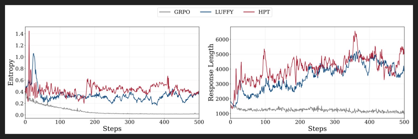
The last thing I want to note is how this model preserves entropy.
Briefly, entropy is a measure of the model’s willingness to explore, as in our explore-exploit dynamic from earlier. Too much entropy is unconstructive of course, but too little means you miss out on some solutions outside your exploration zone.
It’s a known issue now that naive RLVR depletes entropy and overoptimizes models, which the left chart shows; the grey line for GRPO descends and bottoms out to nearly zero pretty quickly.
But that little bit of SFT you keep injecting with HPT apparently does wonders for entropy, keeping it pretty steady on average. And that willingness to explore keeps the model more robust, better able to deal with problems outside its RL training.
My Takeaways
SFT will remain useful
Full worked solutions are more valuable than isolated final answers
Data that preserves (or even restores?) entropy could be valuable, but is under-explored
What would entropy-informed RLHF data generation look like, where entropy guides the creation of preference ranks?