


Originally presented as a live talk on October 14, 2026

Background
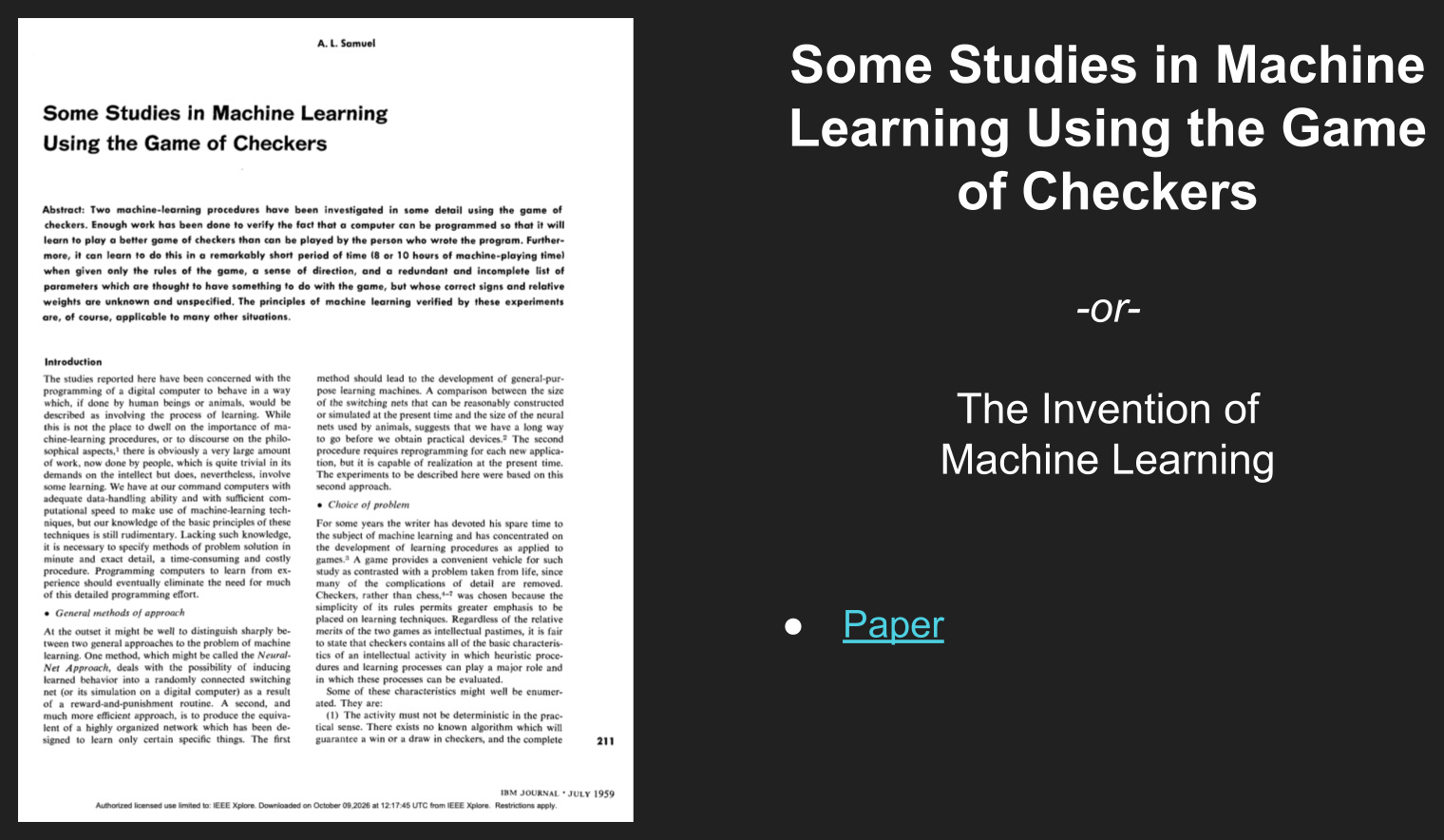
This is an unusual paper for us because it’s not LLMs. It certainly is machine learning though. In fact, the lineage of this paper dates back to the origin of the phrase “machine learning”.
It’s a remarkable paper to read in the present day. The author, Arthur Samuel, has this to say in the introduction:
“At the outset it might be well to distinguish sharply between two general approaches to the problem of machine learning. One method, which might be called the Neural Net Approach, deals with the possibility of inducing learned behavior into a randomly connected switching net (or its simulation on a digital computer) as a result of a reward-and-punishment routine. A second, and much more efficient approach, is to produce the equivalent of a highly organized network which has been designed to learn only certain specific things. The first method should lead to the development of general-purpose learning machines. A comparison between the size of the switching nets that can be reasonably constructed or simulated at the present time and the size of the neural nets used by animals, suggests that we have a long way to go before we obtain practical devices. The second procedure requires reprogramming for each new application, but it is capable of realization at the present time. The experiments to be described here were based on this second approach.”
Did you catch that? He predicted the eventual rise of general-purpose AI based on neural networks almost 70 years ago! What we’re living through now is that first approach he described: large, generic networks for general use.
What he goes on to discuss in the paper is the second approach: a specifically designed network for a single purpose. His network learned to play checkers, whereas the one we’re talking about today learned to play Stratego, but the root idea is the same.
Fun fact: while checkers at the time had no known algorithm mathematically provable to never lose, now it is a “solved game”; a team at the University of Alberta devised such an algorithm back in 2007, after 18 years of work.
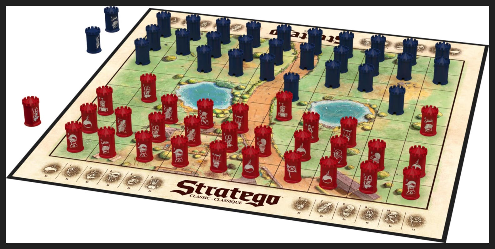
Stratego, on the other hand, is not a solved game. In fact, it is impossible to solve, because the player cannot see everything on the board and cannot feasibly game out every possible scenario. In technical terms, she has “imperfect information”.
Here’s what Stratego looks like for reference. Each player has an array of different pieces, pictured on the key at the bottom. Pieces can generally move one square forward, backward, left, or right at a time. Pieces have different ranks and functions, similar to chess, but when the player’s piece meets the opponent’s piece it’s generally the higher-ranked piece that wins. So if my captain (rank 6) moves to take your piece and it turns out to be a sergeant (rank 4), your sergeant dies. But if your piece turns out to be a major (rank 7), my captain dies. If they’re the same rank, they both die. Crucially, after a battle, the winning piece returns to facing away from the other player, so you have to remember which of your opponent’s pieces you sacrificed a piece to temporarily reveal. There are a few other mechanics, but we don’t need to get into them.
The goal of the game is to capture the opponent’s flag. The player gets to choose the starting arrangement of all their pieces, including the flag, so a big part of the game is deducing where the opponent has placed his flag and his variously ranked pieces.
So while the basic mechanic of moving pieces on a board to capture other pieces is like checkers or chess, the choice of arrangement and the secrecy of placement make Stratego a challenge to model for a learning problem.

In fact, Stratego is such a good choice that there is an existing body of work. The best and most notable entry is DeepNash, by Google DeepMind.
It’s a hefty paper, starting with the author list: 34 folks, including deep-learning heavyweights like David Silver and Demis Hassabis. It also got a hefty budget: 2-3 months of training on 1k TPU nodes, at an estimated cost of $3M-$4.5M. They needed all that compute to complete ~5.5B self-play games, i.e. games between two copies or versions of the same model that bootstrap training data. Those 5.5B games entailed 5-10T training examples, meaning each game was ~1-2k moves on average.
A few million dollars may not seem like a lot now in the age of $2T market caps, but in 2022 it was a serious commitment of resources. It’s about the same as the training cost for GPT-3.
And what did those resources get? Something good, but not something great. DeepNash won 84% of the games it played online, but all the games were one-offs against random people who didn’t know they were playing a bot. When they brought it to the world championships in 2023, it went 19-9 but lost to most of the top-ranked players. There was no equivalent of Kasparov vs Deep Blue or Lee vs AlphaGo, with one master player playing a series against the same bot.
Now you might be wondering why it matters whether a computer is good at Stratego, or chess, or any game really. Why do researchers care about it? Isn’t the goal like, superintelligence and superabundance of material goods?
Well as Arthur Samuel noted in his seminal paper, games are a nice proxy for many real-world problems. If you can make a model that perfects checkers, that can obey simple rules and learn good heuristics, maybe it can spot spam or classify expenses. If you can make a model that plays Space Invaders, maybe you can make a model that controls a robot arm. If you make a model that builds in Minecraft, maybe you can make a model that folds proteins.
In fact, before the dawn of generative AI, a lot of the same researchers and companies were working on AI for games. DeepMind, starting from before it was Google DeepMind, mastered Atari games, then Go, then chess, although they didn’t quite master Stratego as we saw. OpenAI made a model that played Dota at championship level. Before LLMs really took off as the main use case for AI, RL for games and game-like environments was kinda the main thing many AI research labs did.
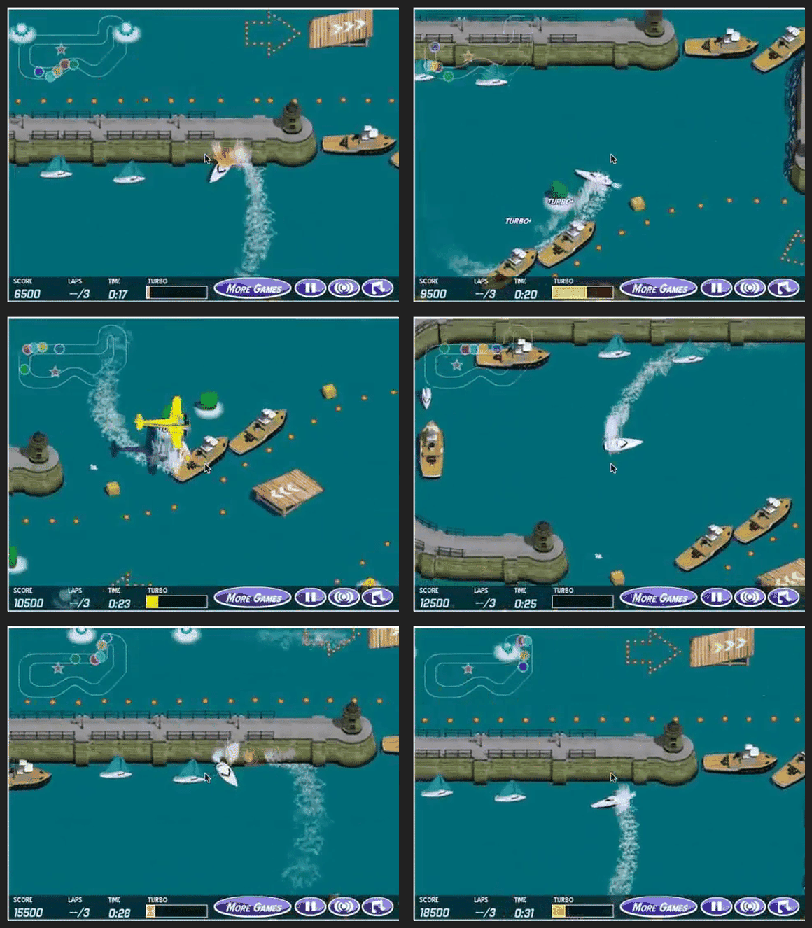
Even Dario Amodei, while at OpenAI, worked on games. This gif is from his classic study on reward hacking, where the model driving the boat in the game CoastRunners learned to rack up points not by winning races, but by hitting the same buoys over and over again. It’s a good example of how games can pull out the principles of machine learning. They are clean, controlled demonstrations for ideas that could work in production. Think of them as the lab rats of AI.
Of course, a wargaming AI might be directly relevant for war. No surprise then that today’s paper got grants from the Office of Naval Research.
So that’s some of the broad-strokes history. Now I want to get into the technical background.
The foundations of the paper are transformers and reinforcement learning, which we are familiar with from LLMs. However, there are several differences between even the basic LLMs of today and the models in this paper. I’ll describe the specifics once we get into the paper itself, but here I want us to un-learn some stuff from LLM defaults.
First is the architecture. We’re going to keep the transformer, i.e. the attention plus feed-forward network composing the transformer block, but we’re going to see three different variants: encoder only, decoder only, and encoder-decoder.
The difference comes down to how attention works. In our modern LLM framing, we expect causal attention, where each token is only allowed to attend to the previous tokens. That’s decoder only, and it makes sense when your goal is to keep predicting the next token, as modern LLMs do.
The opposite of causal attention is bidirectional attention, where every token in the input attends to every other token, regardless of position. That’s encoder only, and it’s good for cases where you just need to understand the input. The classic example here is sentiment classifiers: input a tweet or a product review or whatever, output a sentiment label.
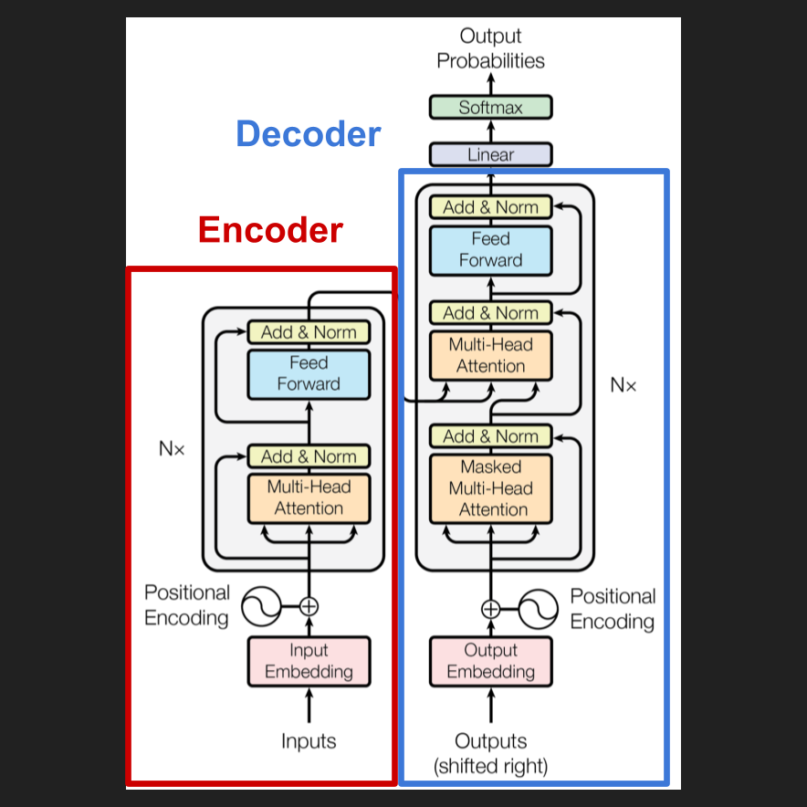
You can stack the encoder and decoder too, and have the decoder causally attend to the encoder’s outputs plus the tokens the decoder itself has output. Actually, the first transformers did exactly that. Here’s a diagram of the original transformer: encoder on the left, decoder on the right. Note how attention for the decoder says “masked”, while for the encoder it does not. That’s because for causality, you need to mask out any tokens in the future relative to the token you’re attending to.
It makes sense on its face; encode your input with bidirectional attention, then generate your output token-by-token with causal attention. So why are modern LLMs decoder only?
It turns out that decoder only is better for scaling up, since you can treat all text as training data rather than separating parts into inputs and outputs; take a big block of text, make the first token the input, predict the next token as output, tack the next token on as input, repeat. In the age of trillion-token pretraining, decoder only wins.
However, in cases where input is clearly distinct from output all the time, having an encoder still helps. The modern example here is in multimodal; since images and audio are always part of the input and not predicted in the output, multimodal models use encoders. However, the text part is still decoder only.
We are going to see all three types of transformer in the paper, so just remember: encoder = look at everything at once, decoder = look only at past and present tokens, encoder-decoder = look at all of input at once + past and present tokens of output.
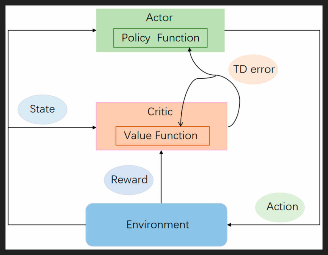
Now that we have our architectures nailed down, we can talk about reinforcement learning.
High-level, I always found RL intuitive: look at outcomes, score them, use the scores to, well, reinforce what’s working. Pretty relatable stuff.
However, once you get into the weeds it gets pretty gnarly fast. The jargon in particular I find dizzying, built up and mutated as it is from decades of work. So I want to provide a glossary of sorts, to help map the abstruse onto the intuitive and familiar. That will help us immensely in the paper.
The first term of RL art is “policy”, or sometimes “policy network”. This is the model in question, the one you want to train to get better. In the context of RL for LLMs, you do hear them called “policy models”, but not really otherwise. The policy network proposes “actions”, like moving a piece on the board or producing the next word in a response. In many cases, an action is a token, but it can also be many tokens.
In contrast to the policy network, we have the “value network”, also called “value function”. As the policy takes actions, the value network provides an estimate of the value of the current state and of the value of the proposed action from the policy network. The value of the proposed action relative to the baseline state is the “advantage”, which usually is what actually goes into your training algorithm. Because of the relationship between the policy and value networks, sometimes they also go by the names “actor” and “critic”.
Two things to note about value networks that can trip up folks coming from modern LLM training. One is that the value network may or may not be different from the policy network. In the latter case, you have a shared model with two different “heads” on it: one for proposing actions, another for outputting values.
Two is that values are not the same as rewards. Rewards are definite and based on the current state of the environment, whereas values are estimates based on the expected end state. Usually rewards come at the end when there is an outcome to evaluate, but intermediate rewards are somewhat common, and process reward models exist for giving out rewards at every step of a trajectory.
That covers everything in the diagram except “TD error”, which basically says how accurate the value function’s estimate was. It can be pretty fiddly and requires balancing definite, far-off rewards with estimated, near-term state values. Important parameters, but too granular for us today.
The Paper

Let’s see how the authors finally cracked Stratego using RL.
Their system, Ataraxos, comprises three models: one for the player’s initial setup, one for guessing the opponent’s board, and one for making moves.
First is the setup network. It is decoder only, since there is no initial input; the player’s side is initially empty, and the policy’s job is to fill it, one piece at a time.
The entire network is only four transformer blocks deep, for a total of 12.6M parameters. Now that may sound shockingly small for folks in LLM land, but you have to remember, these are not general intelligences; in fact, the only “language” the setup network here can “speak” is the twelve different Stratego pieces. It doesn’t even need to explicitly note the positions, since it spits out tokens in board order, from the top-left to the bottom-right of the player’s side.
Actually, there are two other outputs: the conditional outcome and the entropy. The conditional outcome says how likely a win, loss, or draw is given everything placed so far. The conditional entropy says how random the setup is, which is strategically useful for repeat games against a human opponent who would otherwise pick up on the machine’s patterns.
We’ll talk about training later on. First, let’s check out the architecture for the remaining two policies.
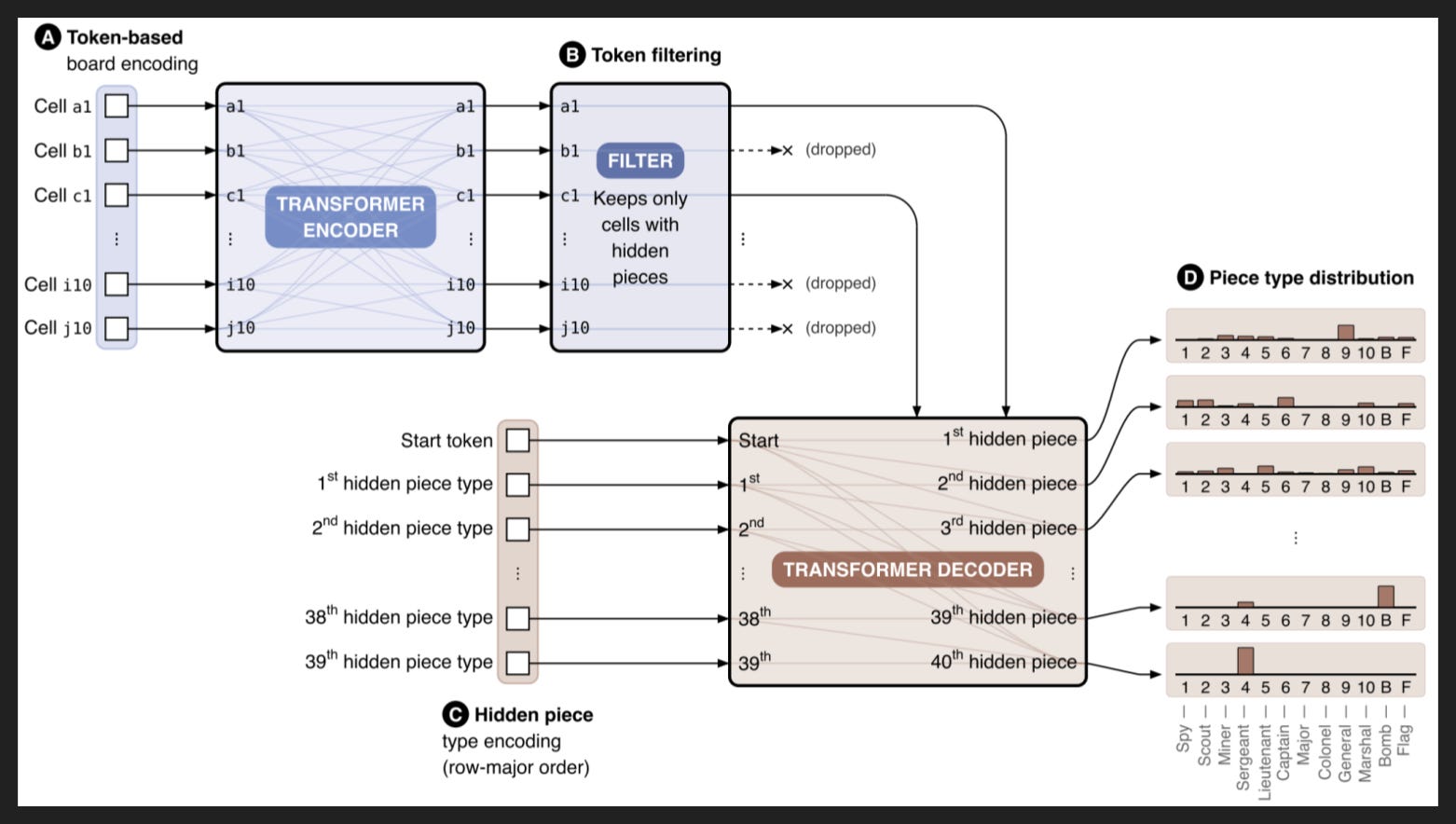
Okay, now this here is the belief network. The belief network is crucial because Stratego is a game of imperfect information. Ultimately, I think it’s the most important innovation in the paper, although more mundane changes to the learning algorithm get more love from the authors.
Conceptually, after the initial setup, the flow of the game is just alternating inferences from the belief and move networks: predict the opponent’s board, make the best move given the predictions, observe any new information from that action about the opponent’s board, repeat.
Architecturally, because the belief network has both an input distinct from the output and must produce many tokens that depend on each other, the natural choice is encoder-decoder. Size-wise, it’s six blocks for the encoder and four blocks for the decoder, weighing in at 57.1M parameters total. It’s by far the biggest of the three, but still tiny compared to even the smallest LLMs.
Anyway, for the encoder component in blue, we see tokens for every square on the board as inputs. Each input token contains information relevant to that position: the current piece in it and that piece’s move history, recent events within the square itself, and some global information like the number of turns left. After the encoder is a filter that keeps only opponent pieces with unrevealed types. The keys and values then become input for the decoder.
Speaking of, the other input for the decoder is a list of all 40 opponent pieces. Each input token has two pieces of information: the type of the previous piece in the list, and the list position of the current piece. So let’s say for piece 0 that we predicted Bomb. Then for piece 1, the information is basically “piece 0 is Bomb” and “this is piece 1”.
Like with the setup network, the belief network decides on its belief of the opponent’s board one piece at a time, just like how a decoder only LLM decides on the next token one at a time. Also just like an LLM, the end result is always a distribution over all tokens.
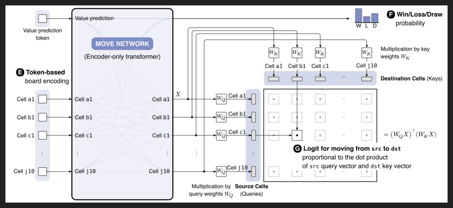
Finally, we have our move network, which says what square to take from and move to.
I phrase it that way, instead of phrasing around which piece to move, because of how the model actually works in the end. But let’s start from the beginning.
The network itself is eight blocks deep. It contains 14.7M parameters, which is a bit bigger than the setup network but much smaller than the belief network. One possible reading is that inferring your opponent’s board is the hardest part of Stratego, which checks out to me. The authors note they needed to keep the move network small since it runs more frequently during inference than the belief network and their ultimate constraint is compute, but it’s impossible to say how big either network would be if compute weren’t the constraint.
Since the move network only needs to return one thing - the move - the natural setup is encoder only. The input is the entire current board, plus a special token at the start called the “value prediction token”. Basically, it’s a place for the move network to store information that isn’t specific to a single square. In the end that token is going to return the likelihood of a win, loss, or draw given the current state of the board and future possible moves.
Now for the rest of the tokens, again they contain information about what piece is currently in them. After the layers of the move network they’re going to combine in a particular way to recommend a move. Specifically, they’re going to form queries and keys, which will multiply in the classic transformer way to produce attention scores. The query is the source square, the key is the destination square, and the attention score is the strength of the recommendation. It’s exactly like the attention operation in an LLM, where the query of one token and key of another combine to say how relevant the key token is to the query token.

So this is normally the place I would talk about data, us being at Scale and all. But once again, we diverge from the typical LLM methods.
With an LLM, you would first pretrain on a ton of unlabeled data, from the internet and from books and from codebases and so on. Then these days you would midtrain on a ton of agentic data - trajectories and so on. And then you would post-train with labeled data: prompt-response pairs for supervised fine-tuning (SFT), prompt-final answer pairs for reinforcement learning with verifiable rewards (RLVR), prompt-rubric pairs for rubrics, prompt-preference rank pairs for reinforcement learning with human feedback (RLHF), and prompt-environment pairs for reinforcement learning environments (RL envs).
For models like in Ataraxos, we have to throw most of that out. All we are doing is SFT and RL on data from self-play, and mostly not in a form that maps directly to LLMs.
To be clear, that means no pretraining at all. Which is actually what allows this project to work in the first place for a team of academics; instead of spending millions of dollars on a months-long pretraining run using hundreds of thousands of GPUs, they spent less than $8k on like a week of RL training using 16 GPUs.
The RL training they did do is like a mix of RLVR and RL envs. It varies by model. So for the setup network, it’s pretty much RLVR: the “prompt” asks for a board setup, and the “final answer” is the game outcome. The reward is 1 for a win, 0 for a draw, and -1 for a loss, with a bonus for entropy to discourage predictability. Note that the advantage is the reward minus the expected outcome, but in self-play the expected outcome should always be close to zero. They run ~163M self-play matches, and both players are the policy, so that means ~326M examples to train on.
Here’s the result of all that training for the setup policy. For each piece type, we see how often we find that piece type in a given setup. Note that most piece types have multiple pieces - four captains, five miners, eight scouts - but for spy, general, and marshal there is only one. Apparently putting the flag in the back corner is uncommon for championship-level Stratego players, but Ataraxos strongly favors it.
Now you might think based on how Ataraxos works that the belief and move networks are part of the same training loop, just as they are part of the same inference loop. But actually, belief network training is a separate, SFT-like step, after the RL for the setup and move networks is complete. Again, working against LLM intuitions.
So let’s tackle the move network and come back to the belief network after. Move network training is most akin to RL envs, where a policy takes actions in and receives rewards from the environment. There are many turns, the environment is only partially observable, and the reward comes only at the end of the game/trajectory.
It’s a bit weird though, because the opponent’s move policy is a big component of the environment! Not only must your move effectively impact your opponent’s pieces, it must also minimize the amount of information about your board the opponent can infer.
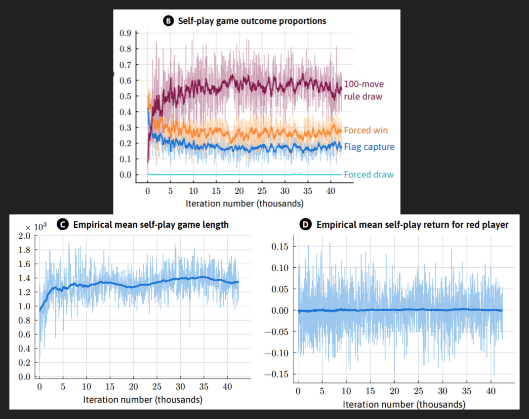
One consequence is that during self-play, which is where all the training happens, the majority of games end in a draw due to hitting the maximum number of turns without a battle. Also, the player version of Ataraxos (as opposed to the generally frozen opponent version) barely has a winning record. Compare that to a typical LLM-powered agent training in an RL env, where you expect rewards to go up over time and to eventually nail the task.
Self-play overall is trickier than the RL env training we’re used to because the opponent is dynamic. One resulting issue is cyclical behavior rather than genuine progression, like learning to throw rock because your opponent throws scissors but then learning to throw scissors because the updated version of your opponent now throws rock. The authors mention strategies to mitigate self-play issues, like adding in randomness and making progressively smaller updates over the course of training, but we will gloss over most training algorithm details.
Overall they collect and filter down to ~50B moves with enough advantage to be worth training on. That’s over 100x more data than the setup network, but it’s much noisier; any single move in a game between two evenly-matched players is unlikely to strongly impact the outcome, and estimating that advantage in a game spanning over 1k steps is guesswork at best.
So now we have a highly competent player, comprising the finished setup and move networks. Now it’s time to learn how to predict a highly competent player’s board, i.e. to train the belief network.
Belief network training is like SFT. The “prompt” is the player’s piece positions and types, plus the opponent’s piece positions, plus some parts of the game’s history so far. For example, any opponent piece whose type was revealed in combat retains that information permanently in the history, even though on subsequent turns the type is not directly observable. Of course, any opponent piece you defeated is visible in the opponent’s graveyard.
The authors put significant effort into engineering that “prompt” - those “features” as practitioners say - rather than just dumping all available information into it. You might think that’s due to the limited capacity of a sub-1B parameter model, but actually it’s a compute issue. The more stuff in the context window, the more compute it takes to make a single move. For these academics, compute is the bottleneck, so anything they can do to reduce compute needs per move or per game, etc., means more self-play games and more training steps.
Engineering features goes against The Bitter Lesson, but the premise of The Bitter Lesson is that over time increasing compute swamps everything. If you are working just at one moment in time, where compute is fixed, hand-designing features can help. The authors are fully aware of what they’re doing and even cite The Bitter Lesson. The main results of the paper don’t depend on these non-Bitter features though, so they should still be valuable. In fact their general approach - architecture, self-play, training, search - generalizes to other games of imperfect information.
With the belief network in place, Ataraxos is complete. Setup behavior in testing is the same as in training, but move behavior is different thanks to the belief network. Specifically, Ataraxos can now use search.
Again harking back to The Bitter Lesson, search is a powerful ML method because it scales with compute. But search isn’t straightforward in a game with imperfect information; for Stratego, you can’t even complete one move if it involves a battle without knowing private information. The belief network is important because it provides a reasonable substitute for that private information and allows search to continue, simulating many moves ahead.
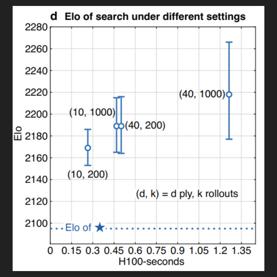
The graph here shows the result. With no search at all, the Elo tops out just below 2100. With increasing breadth and depth of search - rollouts and plies, respectively - Elo ranges up to 2200+. At high numbers, improving Elo increases in difficulty exponentially, so gaining 100+ points is significant. For reference, it took the last 70% of RL training to go from 2000 to the final RL score as shown by the dotted line.
Once the researchers had their completed models in hand, of course they tested against earlier versions and some other bots and random players online, but those evals are no fun.
The real fun is playing a series against a skilled human. In fact, they had Ataraxos play against the best human - a Dutchman named Pim Niemeijer, widely acknowledged as the best Stratego player of all time.
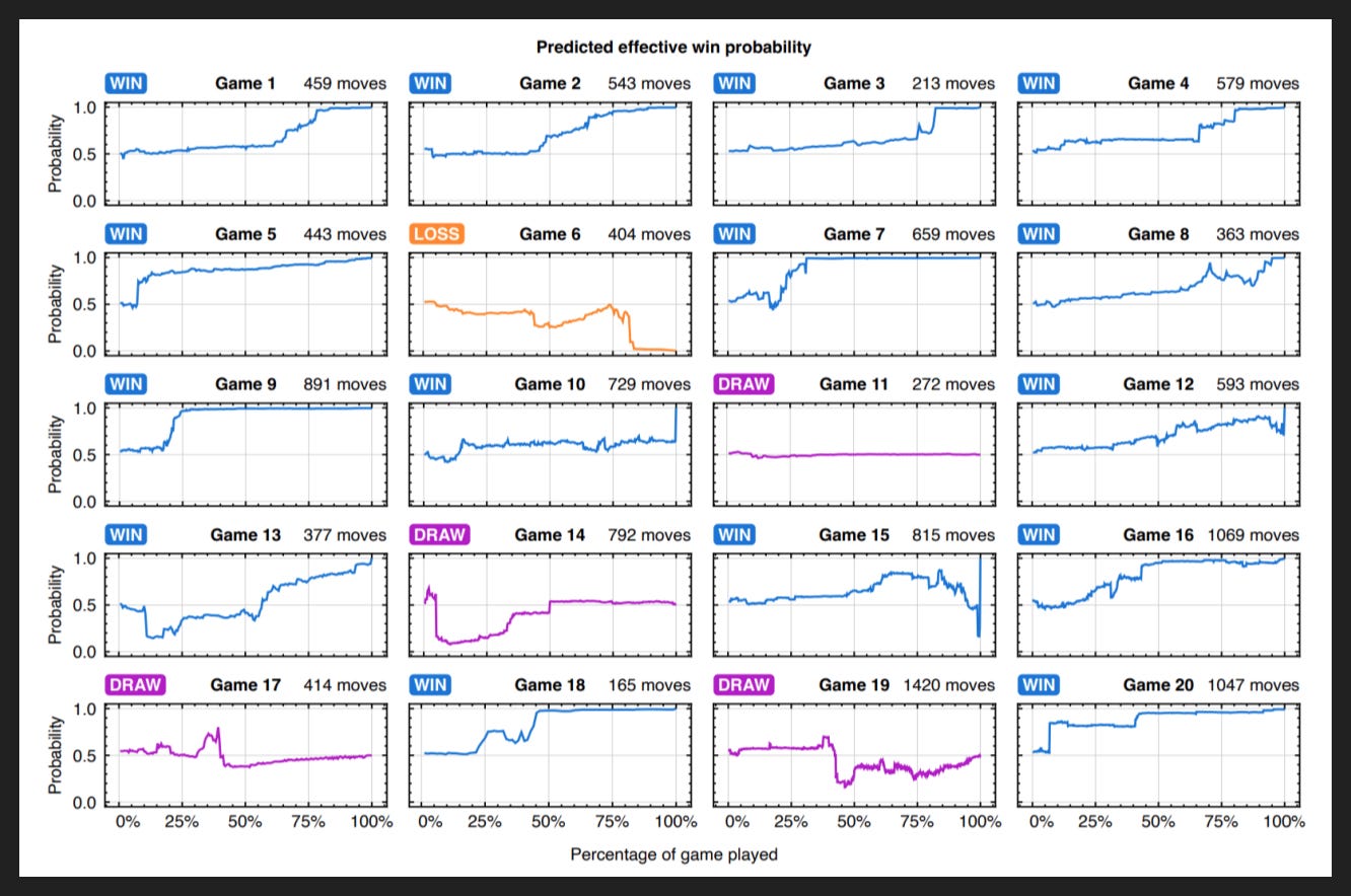
Ataraxos played 20 games against Pim. Of course, Pim learned from each game, but Ataraxos did not; its weights were frozen. Despite its opponent having a learning advantage, Ataraxos was unpredictable enough over the 20 games to avoid giving much ground. It’s true that Ataraxos only won 6 of the last 10 compared to 9 of the first 10, but losing only 1 out of 20 is still the headline result.

Just for some flavor, here are the 20 setups Ataraxos used. The flag is always in the back row and always touches at least one bomb, but otherwise not much repeats.
Qualitatively, some world champions made the following observations about Ataraxos’s play relative to elite human play:
It does a better job disguising the identity of its pieces
It makes more high-variance bluffs and takes more “arrogant” risks
It stalls and employs “rude” tactics when it is behind in order to force a technical draw, i.e. a draw due to hitting the cap on the number of consecutive turns with no combat
It excels at strategies that take a relatively high number of turns to complete
So Ataraxos plays in some alien ways. Although it cuts both ways; to Ataraxos, human play seems alien. They actually incorporate that idea when training the belief network, with a technique called “dropout” that improves performance on out-of-distribution inputs. Since Ataraxos only learns through self-play, it risks not predicting human boards very well.
I want to conclude with the final sentence from the authors about play style: “Ataraxos feels preternaturally lucky, always seeming to have the pieces it needs in the right places, to have its gambles pay off, and to have its opponents do as it wants.” (Emphasis theirs.)
That’s what ASI feels like. Ataraxos is not general intelligence, but it is superintelligence.
My Takeaways
The Bitter Lesson is undefeated
More and better search produces results
Are you making full use of agents and the power of search?
There is plenty of juice left outside of LLMs
As we saw with Jev and the ensuing spurt of decision models, some work LLMs can do is better left to specialist models
AGIs will train specialist AIs
And they will be major consumers of GPUs
We will all be Pim in our own domains sooner or later
Will we all pull a Lee Sedol and retire?