


Originally presented as a live talk on September 3, 2025

Background
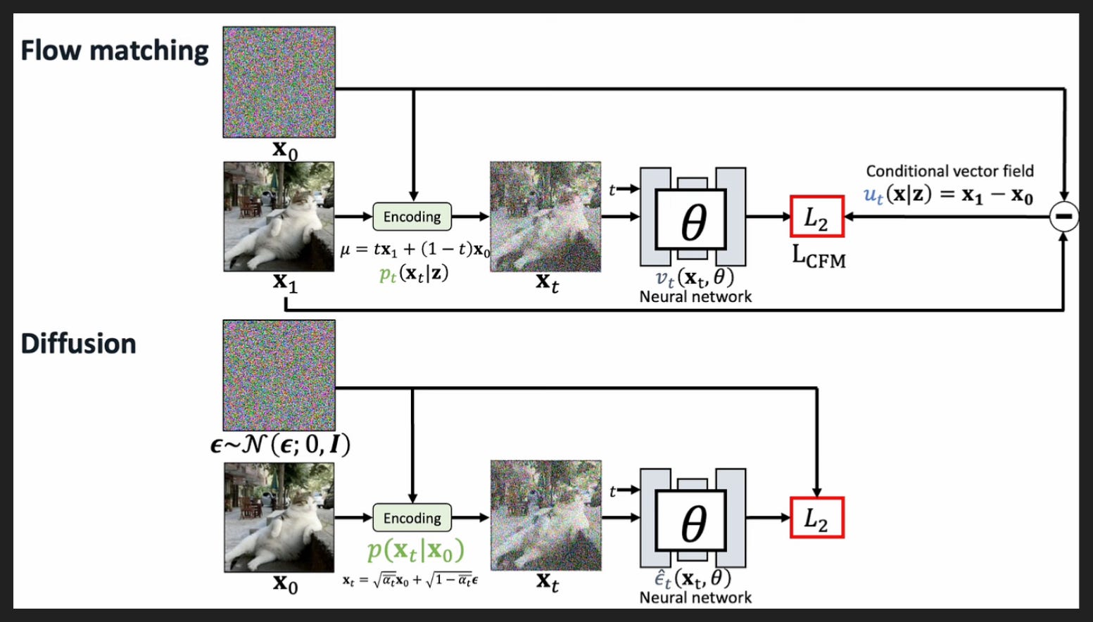
To understand image generation models like Qwen-Image, we need to look at two popular image generation techniques: flow matching and diffusion.
They share some key concepts, so we’ll start with that shared base.
The first concept is signal and noise. Here, signal is a complete, coherent image, like the cat picture marked as x_1 on top and x_0 on bottom. That’s what we’re training the model to reproduce from scratch. Noise is the static-looking box above the cat, which again is labeled differently in the two sections but is really the same thing - random values, typically drawn from a normal distribution as the bottom label for the noise shows - that capital N means “normal distribution”. When we’re training, we know what signal we want to find from the noise because we have the final image already, plus the prompt that goes with it. When we’re actually using the model to generate new images, we’ll start with noise, and the prompt will tell us what signal we want the model to find. It’s sort of like how a carved statue is “in” the stone it’s carved from, you just need to make the right edits.
The second shared element to discuss is time. Now we’re not talking about wall time here, like there’s no measurement of seconds and minutes etc. “Time” in this context is more like steps, so the model gets a certain number of steps to turn pure noise into signal, into a desired image. When you see t in here, that means something is a function of this weird “time” element. And you can see the image labeled x_t in both sections is like an intermediate image between the noise and the signal, the final cat picture. That’s supposed to show that a step along the way from start to finish, from t = 0 to t = 1 usually, is going to have some noise and some signal.
We don’t need to examine every element of this diagram, but the gist is that in both flow matching and diffusion you’re training your neural network to turn noise into signal over some number of “time” steps. And the math looks different between the two methods because they frame this task of turning noise into signal differently.
In flow matching, the idea is to learn the pathways your image can take from noisy to good. The relevant framing from physics here is like wind patterns or ocean currents, where you can imagine a little arrow at every point in space that shows where a little particle would move if you dropped it there. So if you can learn this “vector field” as it’s called, then when you start from a random spot with your pure noise image, no matter where you are the vector field will gently guide you to the right place where your image has now become the thing you asked for. The vector field here will depend on your prompt of course, we don’t always want to generate just the same cat image. We would say the vector field is “conditioned” on the prompt.
By contrast, in diffusion the idea is to learn how to remove noise to uncover the image underneath. Here the physics is more like turning time backwards. Imagine you have a neon sign, filled with neon gas of course, and then suddenly the glass disappears. At the start, the neon will be in the exact shape of your sign, but almost instantly the neon will start to diffuse into the air in the room, until soon the neon is evenly dispersed throughout the room. If you then reversed time, you would see the neon un-diffuse and turn back into the sign.
That is basically what diffusion is trying to learn; you show it a lot of diffusion from signal into noise, and it learns how to do the reverse process, turning noise into signal, or “de-noising” as it’s sometimes called. Again, the process will depend on your prompt, so you’re not always generating the same cat image.
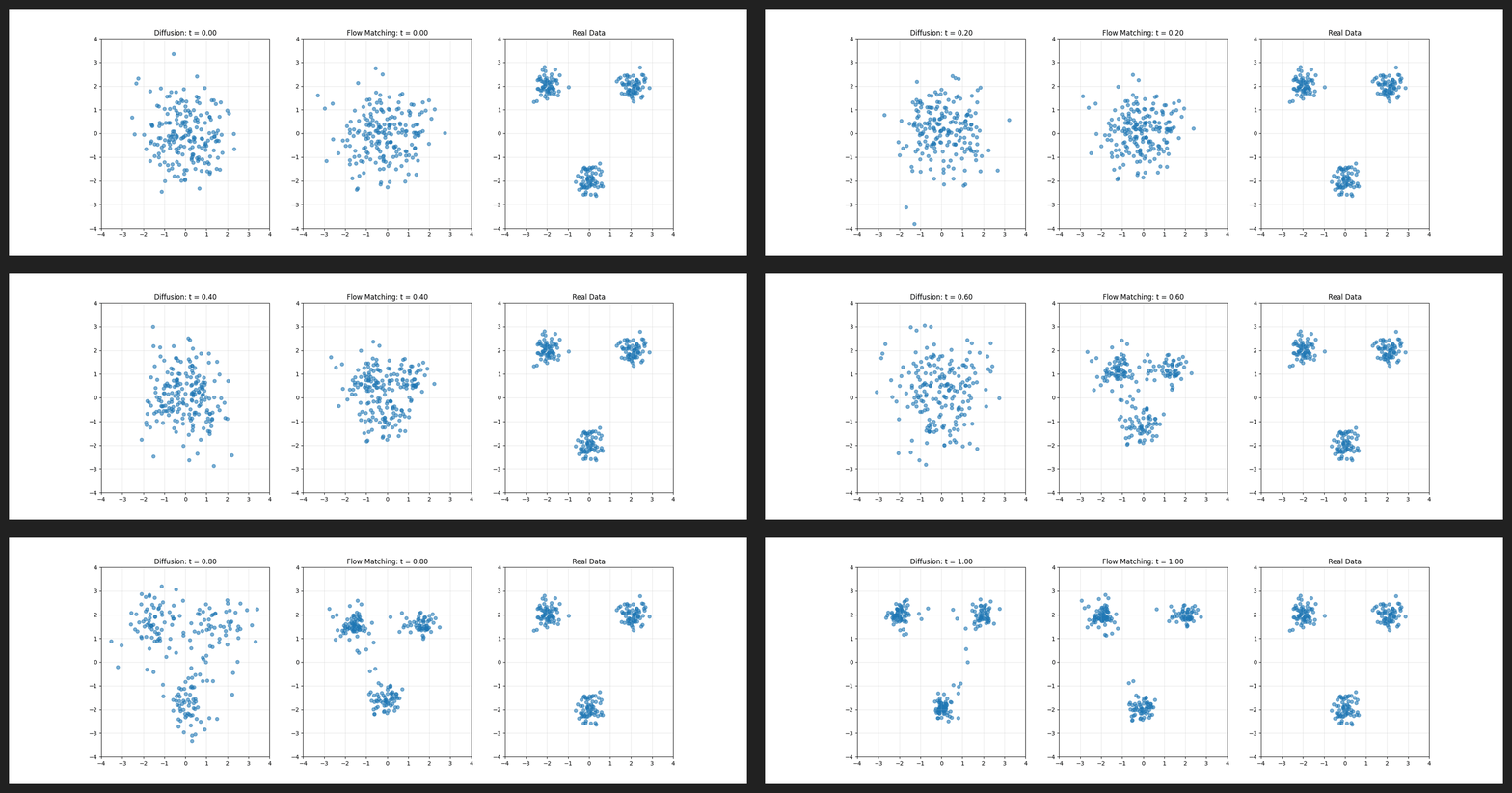
Here’s a little gif showing diffusion on the left and flow matching in the middle, plus the final pattern they’re both trying to learn on the right. As you can see, diffusion and flow matching have pretty different flavors, but they’re both able to land in basically the same place.
This is just a toy example of learning points on a 2D plane, but you could imagine each blue dot as representing an image in the making. The pattern on the right could be the areas of good quality images, which diffusion and flow matching are trying to put their images into.
Note the time at the top! As I mentioned, t usually goes from 0 to 1. Here they’re taking steps in increments of 0.02, meaning the model gets 50 steps to go from noise to signal.
Since Qwen-Image also supports image input, like for editing images, we also need to understand how Qwen-Image understands images.
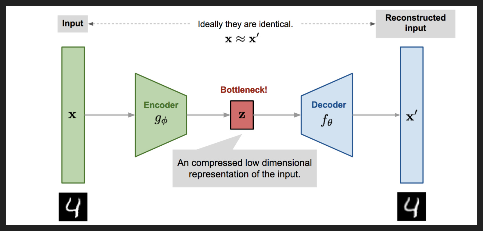
We’ll see a bit later that it uses something called a variational autoencoder, or VAE. It’s a fancy sounding name, but really all it means is it learns to represent images compactly.
We’re all familiar with compression in our day-to-day use of digital systems. For anyone who ever downloaded MP3s, you probably remember the different bitrates - 320 kbps sounds nice, 256 kbps sounds acceptable, 128 kbps sounds pixelated. Well those are all different compressions of the original uncompressed song, made so that a song only takes a few MB of storage, compared to tens of MB for an uncompressed version. To squeeze a song into that little space, the MP3 trades off quality for compressability.
A VAE basically does the same thing, but in a learned way rather than in a preprogrammed way, and for images instead of songs. As this diagram shows, the initial input gets cut down to its essentials gradually by the encoder, until it’s in a “latent space” of lower dimension that is super compact.
You can then decode from that latent space back to normal image space to see how lossy your compression was, which is how you train your VAE to make good representations - if the decoded version is nothing like your input then you have work to do.
And if all you did was encode and then decode, compress and then decompress, then you wouldn’t really be getting anywhere. But if you could encode, then make some changes in latent space, when you decode back out you could get something pretty interesting. Keep that splitting of encoding and decoding in mind for later.
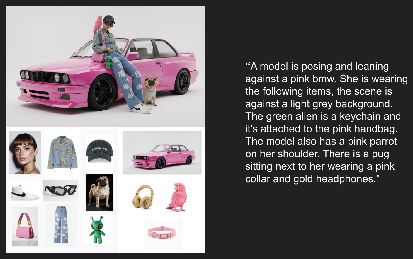
Now more on the deployment side, Google recently released Gemini 2.5 Flash Image, which went by the codename nano-banana on the LM Arena text2image leaderboard while it was still under development. It’s now the undisputed leader there, with a record-breaking lead in Elo score.
One thing people are really blown away by is how well nano banana can combine individual elements together coherently while maintaining consistency for each element. This is an example from Twitter where the user provided 13 input images and a prompt describing the scene, and nano banana was able to create the image as described without altering any of the input items. The prompt didn’t even need any weird tricks to get that consistency - it just described what the user wanted, and the model took care of the rest.
I don’t have much to say about this technically, but just keep it in mind when we’re reviewing Qwen-Image outputs as the high water mark. And remember the two qualities this guy was so impressed by: consistency and coherence.
The Paper
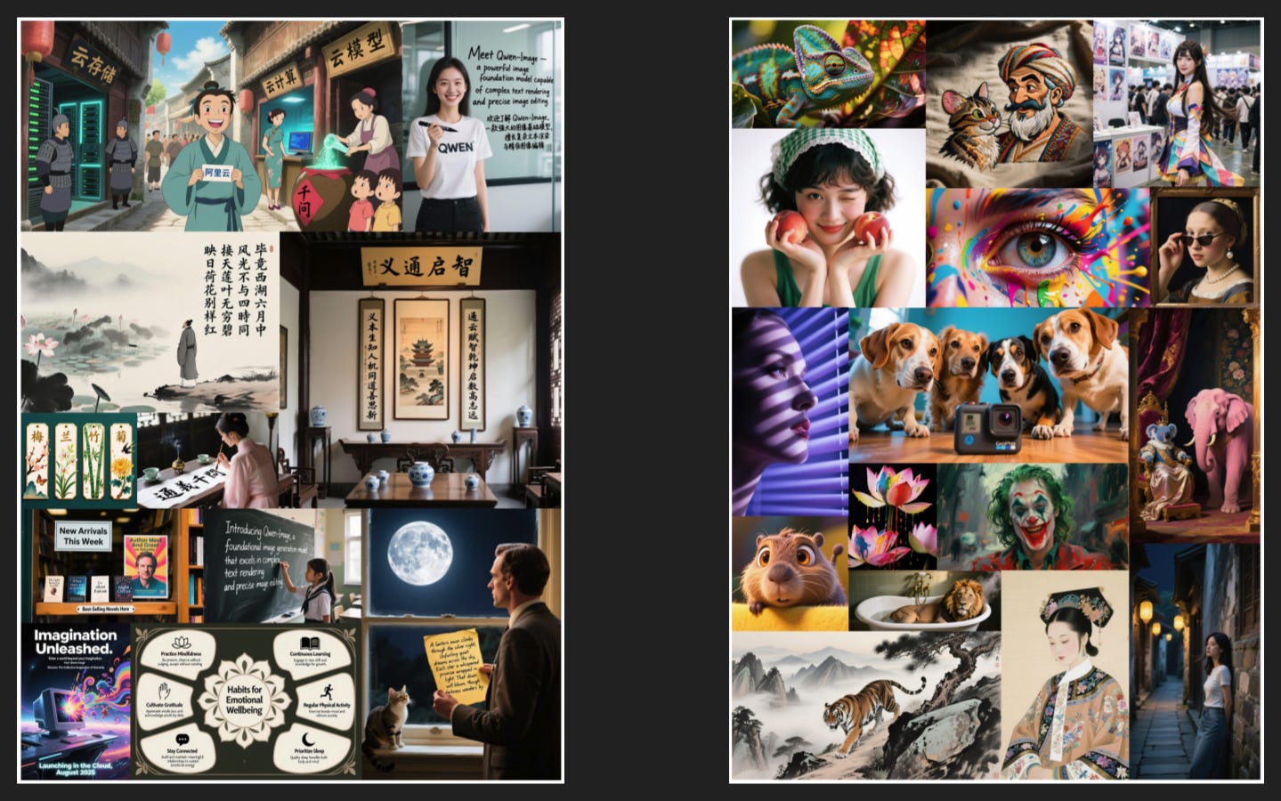
Let’s start by looking at some examples the authors highlight, grouped by skill.
On the left is image text. Now the authors spend a lot of time on this in the paper, but frankly I think a major reason for that is Chinese has been especially tough to get right, and this is a Chinese lab after all. Of course we’ve all had experiences with image generation models where letters get dropped or appear twice or look funny, so I’m not taking away from the impressive text generation on display here. I just don’t want to spend as much time as the authors do on it.
On the right is an array of styles, ranging from photorealism to digital art to painting to drawing to CGI. That’s much more par for the course.
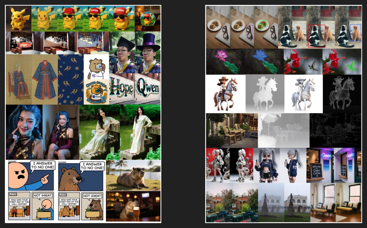
Here on the left is editing, which includes expanding the frame (as with the cosplay) and isolating elements (as with the kimono). I was particularly impressed with the webcomic example in the bottom left.
Finally, here on the right they call “understanding”, saying “detection, segmentation, depth/canny estimation, novel view synthesis, and super resolution - tasks that can all be viewed as specialized forms of image editing”.
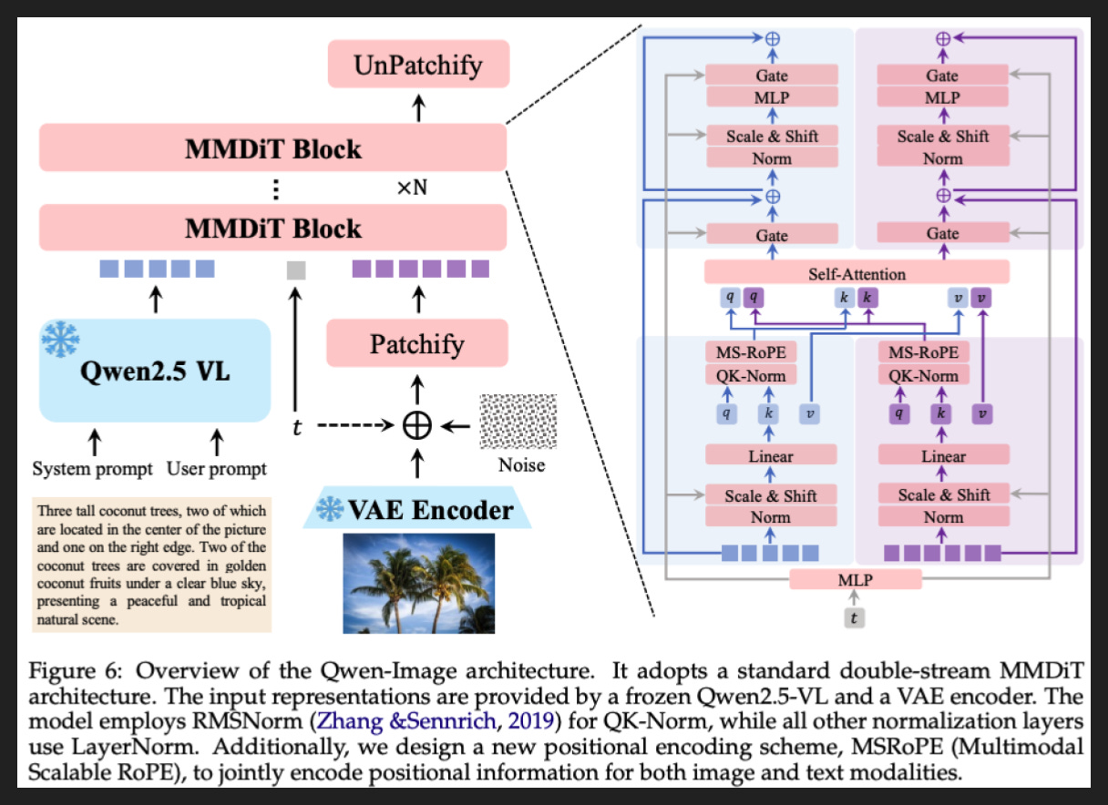
So let’s start diving deep with a look at the architecture of a multimodal diffusion transformer, or MMDiT. Even though it has a fancy name, you can think of it mostly like a LLM with image stuff layered in - hence the “diffusion” part of the name.
Now I know what you’re thinking: “how the hell am I ever going to understand that?!”
But fear not: there are only a few key pieces. A lot of the boxes and lines on here are details we don’t need to worry too much about.
So first, let me provide the key they do not:
The little colored squares are tokens. The arrows show where they go. Blue means text, purple means images, and the grey one is time, in the weird diffusion sense we talked about earlier
The red long rectangles are steps in the information processing pipeline that is a model. The two blue ones are also steps, but they’re “frozen”, i.e. not altered during training
The stuff on the right is what happens in each MMDiT block
The plus sign in a circle just means addition
Now here’s what happens inside a MMDiT.
The text input goes into Qwen2.5 VL to get turned into tokens. The image input, if you’re using it, goes to the VAE Encoder and then mixed with some amount of noise (depending on the “time” t) and the turned into image tokens. Also if you’re using image input, the image goes into Qwen2.5 VL too, which captures meaning and understanding, whereas the VAE captures aesthetics and low-level details.
After that you do the MMDiT block N times. Within each block, you are doing the same steps with the text tokens and the image tokens in parallel, except for one shared step in the middle that we’ll get to.
Anyway, the very first thing you do is actually turn that time t into something other parts of the network can understand, using that MLP at the very start. So once the relevant steps have the time information, they’re ready to go.
Now the text and image tokens move through a few different layers. Norm is a preprocessing step. Scale & Shift is similar but focuses on that time information. Linear is the first real “thinking” step and creates the query, key, and value matrices, which are the inputs into our shared layer, Self-Attention.
Now the query and key matrices get their own special QK-Norm, again a sort of preprocessing, then they get position information added in MS-RoPE, so the model knows what order all the text and image tokens were in. We’ll visualize that technique on the next slide.
So the enhanced query and key matrices, plus the value matrices, combine in Self-Attention. What exactly self-attention is or does is well-covered elsewhere, but for our purposes it’s enough to know that attention is the most important part of a modern model. It’s where the model learns what to pay attention to at any given moment and what all the information really means, a crucial second “thinking” step.
Then after Self-Attention comes Gate, which again takes that time information and applies it to the Self-Attention output to turn it up or down. Our old friends Norm and Scale & Shift return, then comes MLP, which is the third and final “thinking” step. This is where the model transforms the information it understood in the previous steps into something new as it gets ready to produce the next token. And then we have a final Gate to again modulate depending on the time.
So after all that - incorporate time info, preprocess, break into query/key/value, add position information, attend, modulate, preprocess again, contemplate, and modulate again - we’re ready to predict tokens. And if they’re image tokens they get pieced together like a puzzle in UnPatchify. But that’s it! You know how it all works now.
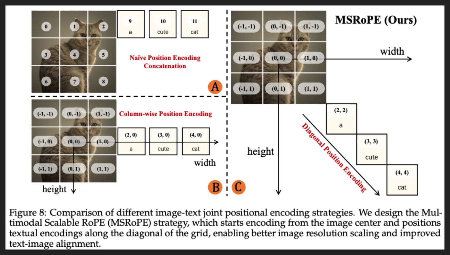
Since they make a big deal out of it, I do want to quickly visualize their positional embedding strategy, MS-RoPE.
I think the easiest way to understand it is to start with strategy A, which is just assigning a number to each image patch and then each text token. That’s probably how humans would like to receive this information if it had to happen one token at a time.
Strategy B is not really important to understand if all this is new to you. Better to just look at strategy C, which is their strategy. Instead of giving each token just one number, they give it two, like a coordinate in the x-y plane. So here they have the origin in the middle of the image. And then they add text tokens along the diagonal, like along the line x = y. And that makes sense because if you drop the image and just have text, then you can just drop one of the coordinates and the text tokens will still have an order that makes sense. So you’re teaching the model with these positions not to favor x or y, to treat them the same. That’s really important for images, where what matters is the relative position between parts of the image, not the absolution position in the height or width of the image. Like there’s nothing special about height vs width, you could just rotate an image 90 degrees and it would be the same image at heart even though height and width would have switched.
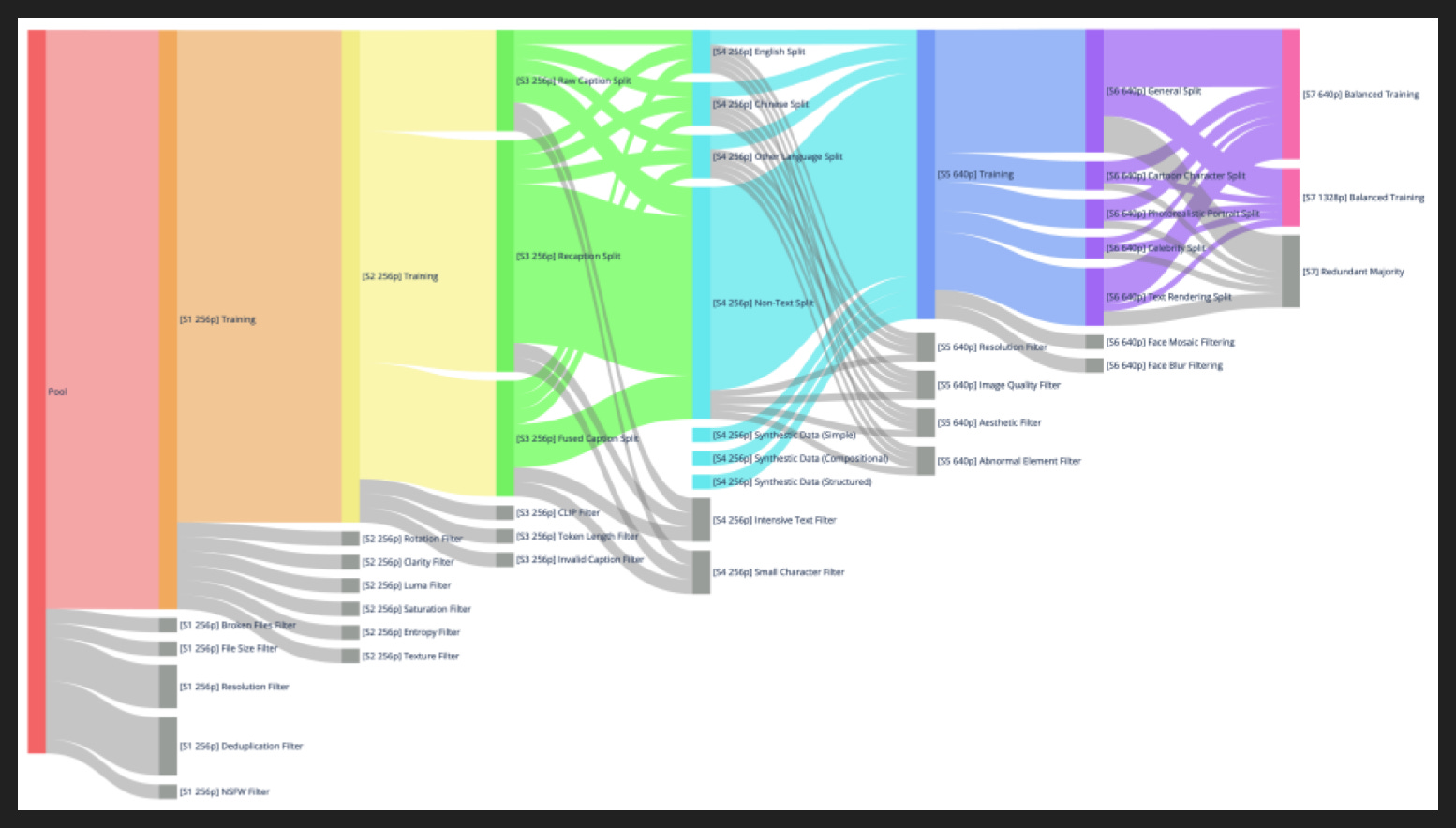
Turning to the pretraining data, they collected billions of image-text pairs, then filtered and balanced out in stages during training. Each of the seven steps here got trained on in sequence, so the biggest but roughest pool to start, then the smallest but highest quality pool to finish, which is now the norm in pretraining.
Here are the seven steps:
Initial Curation (red) - pick a set of minimum pixel count, dedupe, and remove NSFW
Quality Enhancement (orange) - take out images with significant issues like blurriness, or significant editing like flipping or saturation. Also take out low-information images as being unhelpful, and unusually pattern-dense images as likely containing noise
Image-Text Alignment (yellow) - use text-image alignment models to find and filter misaligned pairs. Discard pairs with very long captions or likely caption errors like “No caption found”. They also synthetically generated some captions with Qwen-VL, which provides more image detail but usually misses world knowledge like cartoon character names
Text Rendering Enhancement (green) - split into English vs Chinese vs Other vs No Text, filter out examples with very dense or very small text, then selectively create synthetic examples to balance out the four splits and provide variety in fonts
High-Resolution (light blue) - increase resolution minimum, filter out defects like blur or compression or watermarks, then something they call an “Aesthetic Filter” for “composition or visual appeal”, which I’m not sure how they decide on
Category Balance and Portrait Augmentation (blue) - categorize and rebalance by General vs Portrait vs Text Rendering, and add synthetic captions for portrait-specific details like facial features, which apparently helps with instruction following as well as image quality
Balanced Multi-Scale Training (purple) - add more detailed image taxonomy and balance further, and upsample higher resolution imagest
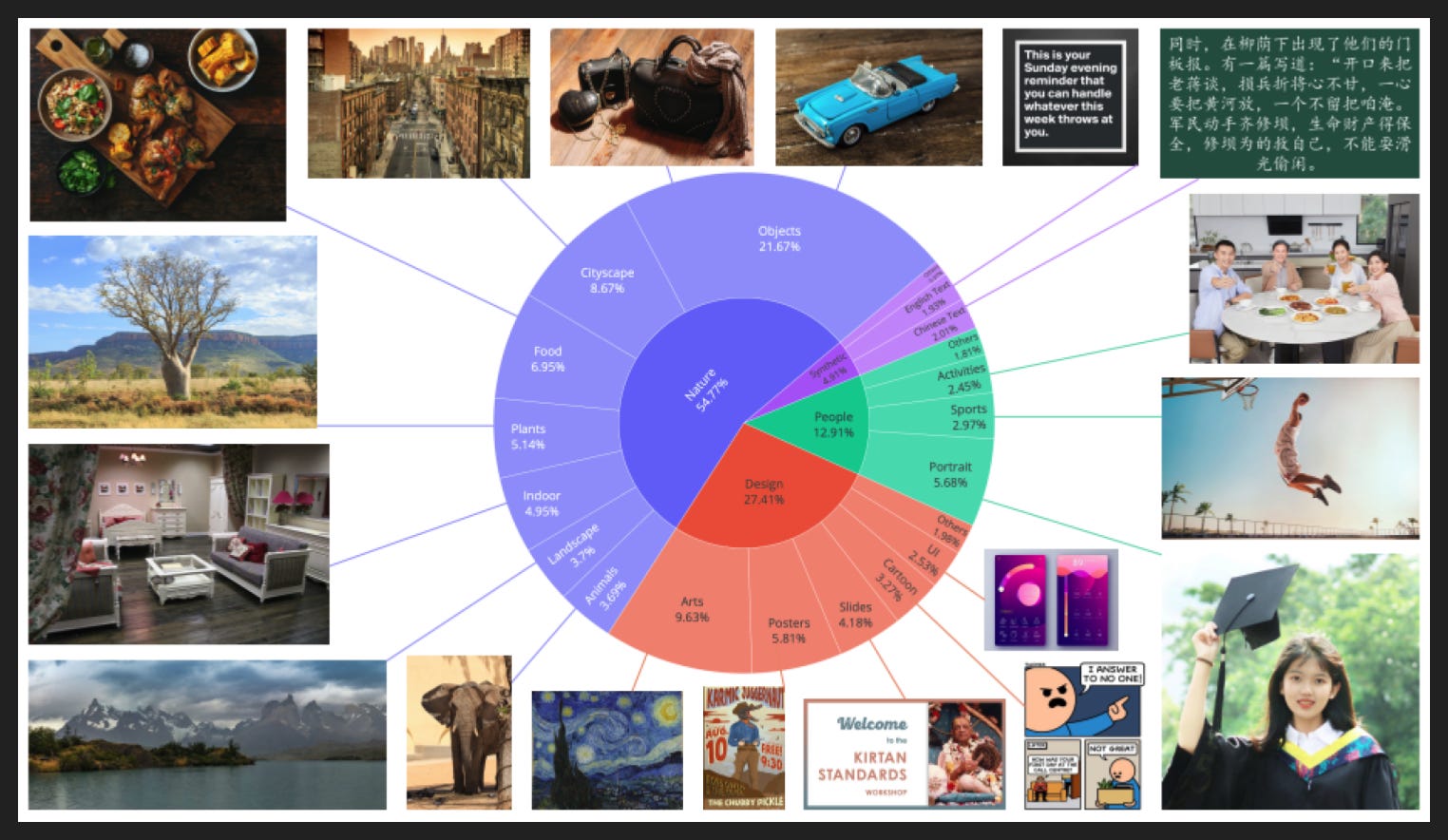
Here’s the breakdown of the final dataset by domain and an example of each.

Now here is where I would describe details of their post-training… if they provided any.
All we know is they did some SFT and some RL, using DPO and also GRPO.
The preference ranks for DPO did use human annotation, but some of the preference ranks used existing reference images as the preferred output, rather than always using two outputs from the same model at different temperatures, i.e. a deviation.
Other than that, we know nothing. There’s absolutely no information about volumes of either SFT or RL data, no performance curves, nothing. So not very instructive for us.
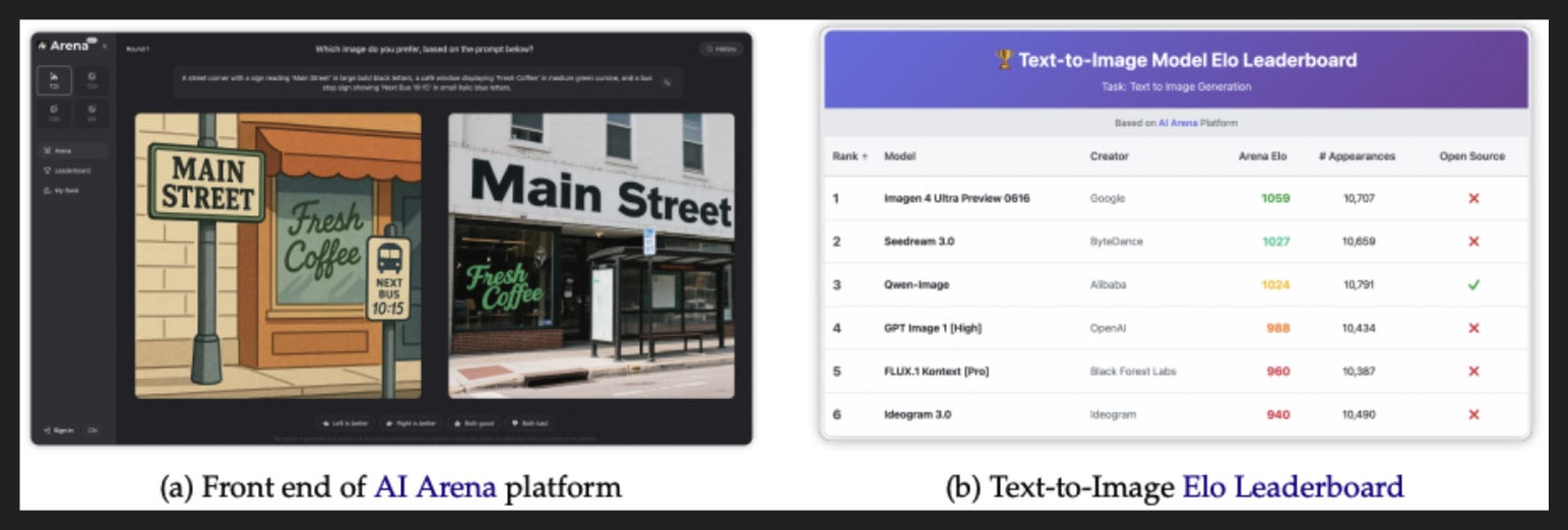
As part of the paper they also made their own version of Chatbot Arena, which they creatively call AI Arena. The live results today basically match the results shown in the paper here, which puts them ahead of GPT!
However, nano-banana is not in the list of competitors, so I think they’re overplaying their hand a little here. Still, GPT image generation seems to be good enough to dominate casual use. To have that “at home” for free is impressive.
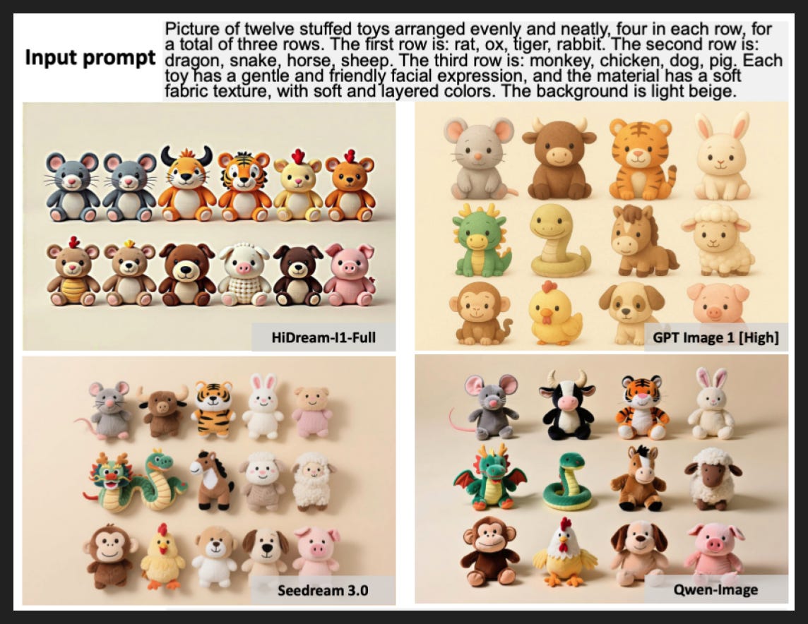
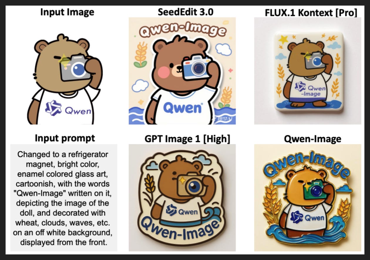
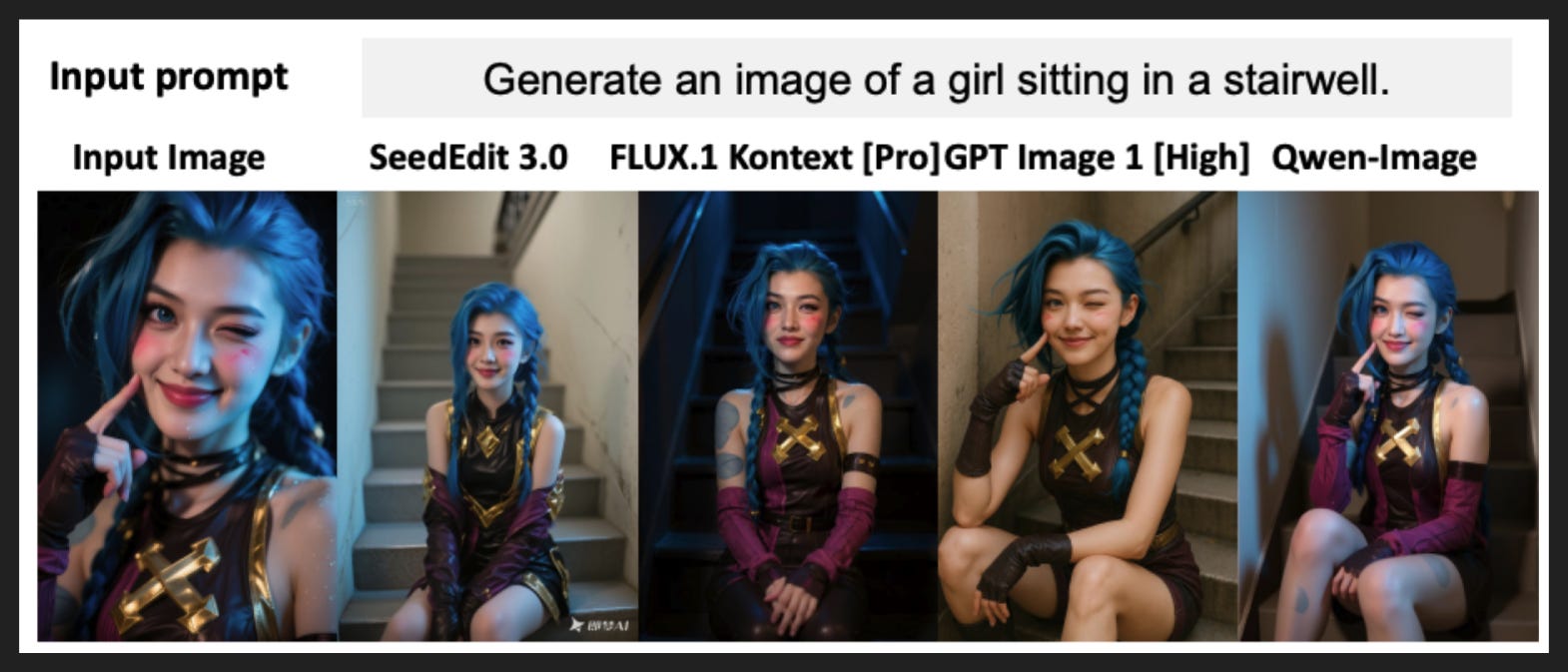
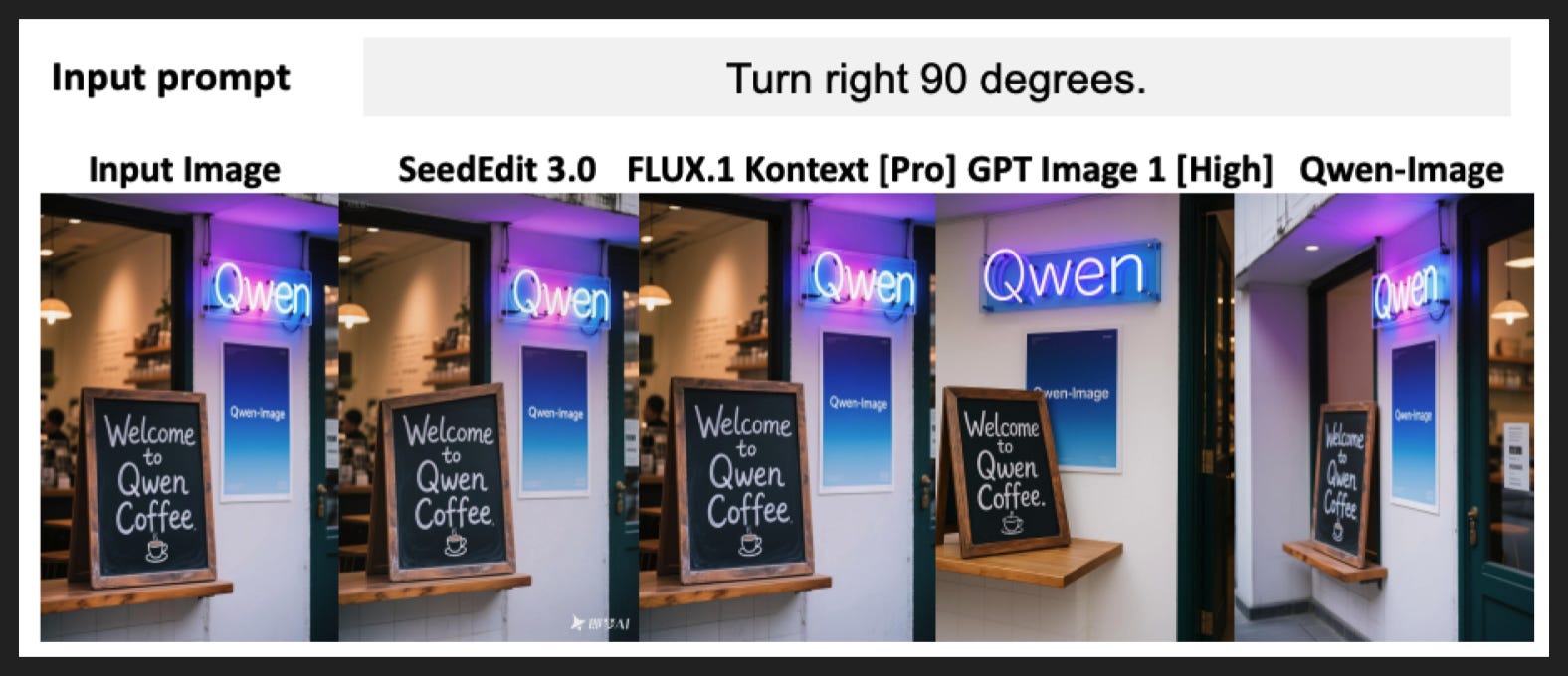
There are a few other qualitative trends called out in the paper, although a lot of it is focused on text which I’m not that interested in. I pulled out a couple of the more compelling examples here, but of course this could all be c-herry-picked or sensitive to the exact wording of the prompt.
I should note they also list more quantitative performance metrics on several image generation and editing benchmarks, which can judge objective things like “is this object in the prompt present in the image” but I think still would do a poor job on vibes. Whatever you make of these measures, Qwen-Image matches or beats the other models on most measures, including GPT.
My Takeaways
Professional-grade image generation and editing is here
We are beyond the Stable Diffusion days where image generation was its own kind of art or just used for throwaway purposes
Editing is an emerging capability worth watching
Generation is harder to evaluate because so many possible outputs are acceptable and taste is such a strong determinant
Editing is more objective and also more reflective of commercially valuable work
Adobe may be in trouble