

mHC vs Attention Residuals

Originally presented as a live talk on April 1, 2026

mHC: Manifold-Constrained Hyper-Connections
or, The Importance of Being Normalized

Attention Residuals
or, Attention Really Is All You Need
Background

So since this is a head-to-head paper review, we have to talk about the two fighters in the ring.
On the left we have DeepSeek, one of the two S-tier labs in China, the other one being the Qwen folks. DeepSeek is an outgrowth of a hedge fund called High-Flyer, and it has spent a lot of its life as a fun science project rather than a hard-charging startup. That culture of exploration has produced some highly respected research, including the birth of the modern MoE model and the public discovery of how to train reasoning models, which previously only OpenAI had discovered with o1 and o3, but kept private.
We covered one of their most recent innovations, the Engram memory system, back in February. The paper we’re covering today, mHC, came out just before that.
Everybody thought DeepSeek would release V4 of their flagship model around Chinese New Year, but that was weeks ago and so far we’ve heard nothing. I suspect the combination of high internal standards and little commercial pressure has them working on improvements rather than shipping something middling.
Now on the right we have Moonshot, makers of the Kimi series of models. Moonshot is a hard-charging startup, solely dedicated to making commercially viable LLMs. They were founded in March 2023. Since then, they have released several versions of Kimi, most recently Kimi K2.5, a 1T parameter model. They also just raised $1B and plan to IPO in Hong Kong soon.
Kimi has won praise for its overall performance, but in particular its personality and writing skills. I think it’s the “Claude-iest” Chinese model, which actually would make sense, since recently Anthropic accused Moonshot of distilling from Claude. Possibly relatedly, Cursor used Kimi as their starting point for their most recent coding model, Composer 2.
On the science side, they traditionally haven’t released a ton, although they did claim some engineering breakthrough related to the optimizer Muon.
Okay, now we can get into the technical piece.
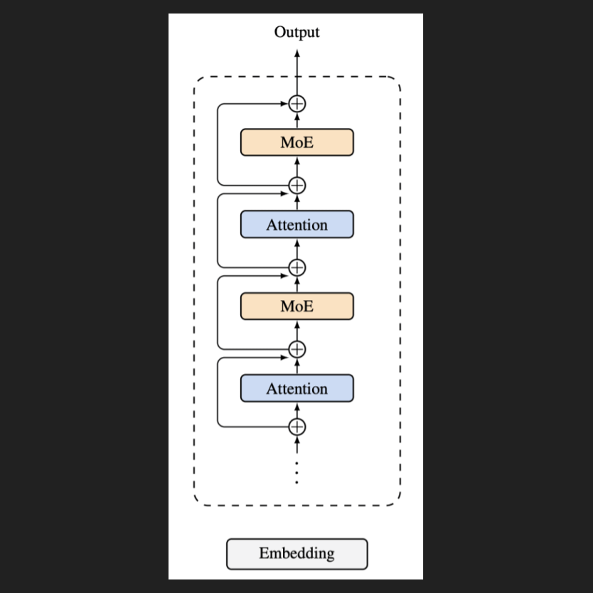
First, let’s recap transformers. To oversimplify somewhat, transformers have three pieces:
Embedding, for turning text or other inputs into vectors
Attention, for understanding how different parts of the input relate to each other and forming a holistic view
Feed-forward network, for “thinking” or processing that understanding. In this diagram the feed-forward network is a MoE, a kind of sparse network. In other transformers it’s a dense network
Embedding happens once at the start, then attention and FFN layers trade off over and over again, dozens of times. One attention plus one FFN layer is called a transformer block. In this diagram though, they only have four layers, and they don’t show the division into blocks.
Now in reality there are other minor components, like RMSNorm or similar, but we will put them aside for now.
The only thing left to note is these arrows and plus signs, which show how information flows and combines between layers. That’s what we need to take a closer look at.
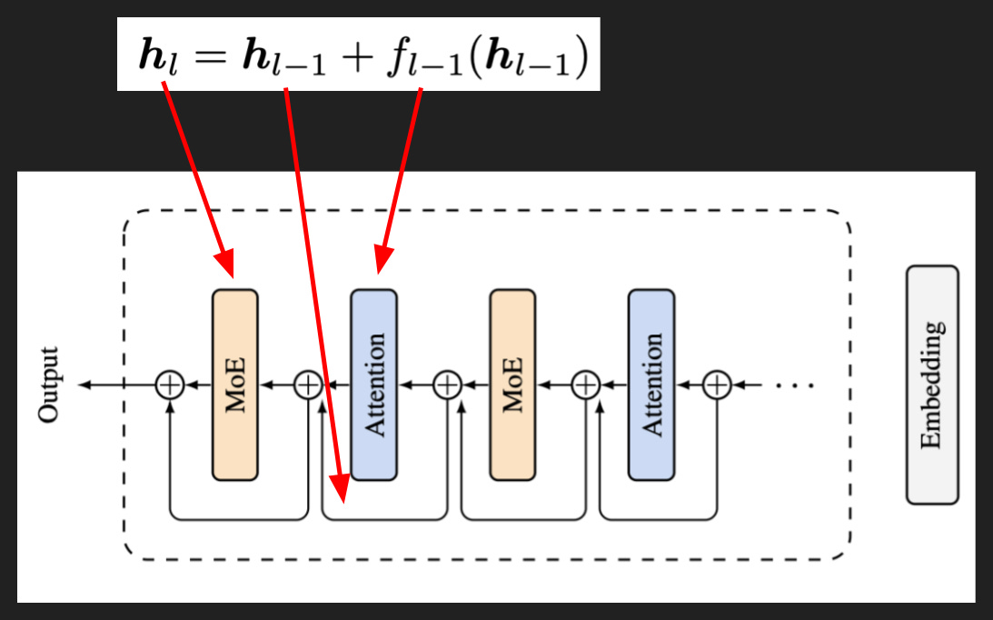
This is where residuals come in. Mathematically it’s very simple, but in the diagrams I used to find it confusing.
Here “h” is a hidden state, basically the stuff that moves along inside a model and that the attention and FFN layers process. Then at the end the hidden state gets turned into a token or a class or whatever other thing your model is predicting.
It used to be that hidden state passed directly from layer to layer, like the output of one layer would be the input of the next layer. But then, back in 2015, some researchers at Microsoft decided to add in this other component, the residual - the hidden state from before the previous layer.
In the formula at the top, that’s h_(l-1), the first term on the right side. The second term is the output of the previous layer, where the function f_(l-1) is either attention or FFN. The little plus sign in a circle in the diagram literally means addition - you are adding the output of the most recent layer to the original input for that layer, and that’s what forms your input for the next layer.
So that’s what residuals are. Now the question is, why do we need them?
To understand that, we have to look at the two directions information flows in a transformer: forward, when you’re doing inference; and backward, when you’re training.
The forward case is more straightforward. If you only have the output of one layer as the input of the next layer, you can lose sight of the original input. It’s like playing a game of telephone - changes and errors can stack up. But if you add the residual connections, you’re always providing an unaltered version of the past layer’s input.
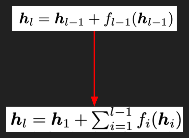
And if you look at the formula from the last slide, you can actually write an equivalent version, which I’ve shown here. Notice in the new version that the hidden state for the current layer relates directly to the hidden state entering the first layer; the current state is the original state plus all the layers. If you didn’t have the residual connections, you would lose that h_1 term. So the residual connections let information flow directly between layers.
So that’s the forward pass. Now for the backward pass, we have to get a little more sophisticated.
When you are making a model, you ultimately are trying to minimize some loss, some formula you’ve written that describes how far off your model is from ground truth. So in a linear regression for example, a very simple mathematical model where you’re just trying to fit a straight line to a series of points on a graph, your errors are the distances between each point and the line, and your loss is the sum of the square of those differences.
Loss for a LLM is really not that different. When you’re doing pretraining or SFT, your loss is related to the probability your model gave for the actual next token in the training data. When you’re doing RL, your loss is related to the rewards you’ve calculated.
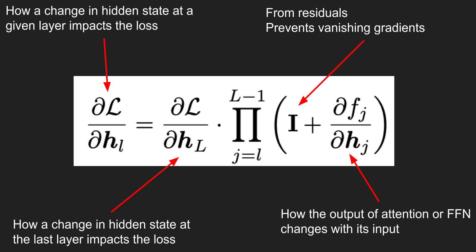
The big script L in this formula is the loss. On the left side, what we’re asking for is how to calculate the change in loss if we make changes to the input at a certain layer. And if you look on the right side, you see that it depends on the changes to the loss due to the input at the final layer, capital L, and the changes to just the attention or FFN outputs at each layer. It’s just the chain rule from calculus, applied to the giant mathematical equation that is the LLM.
Note something important here in the formula though: that capital I, which is basically the vector equivalent of 1. That’s due to the residual connections. And without it, if enough of those local changes are close to zero, then the whole right side basically ends up at zero. This problem is called “vanishing gradients”, and the more layers you add, the more of a problem it will be.
So the residual connections allow your training information, your measurement of how any tweak to the system will impact the loss, to persist.
So that’s your basic residual connection setup. It works great, everyone uses residuals, problem solved. Right?
Well we’re going to see about that in a minute, but one final bit of background to introduce, or perhaps reintroduce, is The Bitter Lesson.
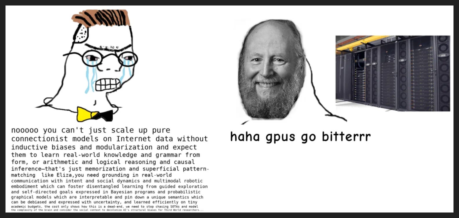
The Bitter Lesson is an essay by famed machine learning researcher Rich Sutton, pictured here as a GPU enjoyer. His basic point in the essay is that because computing power grows so quickly, scaling up “dumb” or simple approaches always beats “clever” or complex approaches that humans design. For example, when a machine beat a human at chess back in 1997, it didn’t have lots of sophisticated chess strategies in its memory; instead, it searched the space of possible moves by brute force, and it just so happens that in 1997 that was finally technically possible.
The same thing is true for the field of machine learning that deals with language, “natural language processing”. People spent a long time trying to encode the rules of human language into machines, but then along comes OpenAI and just dumps an Internet worth of text into a model and throws enough GPU time at it to learn to produce human language.
The way I think of it is, learning surpasses engineering. If we can learn something rather than design it, we should.
The Papers

So both papers want to change how residuals work. They just disagree on the best way to do it.
I’m going to reground us in the two forms of the residuals equation from Moonshot: recursive, on the left; and iterative, on the right. Remember, these are mathematically equivalent.
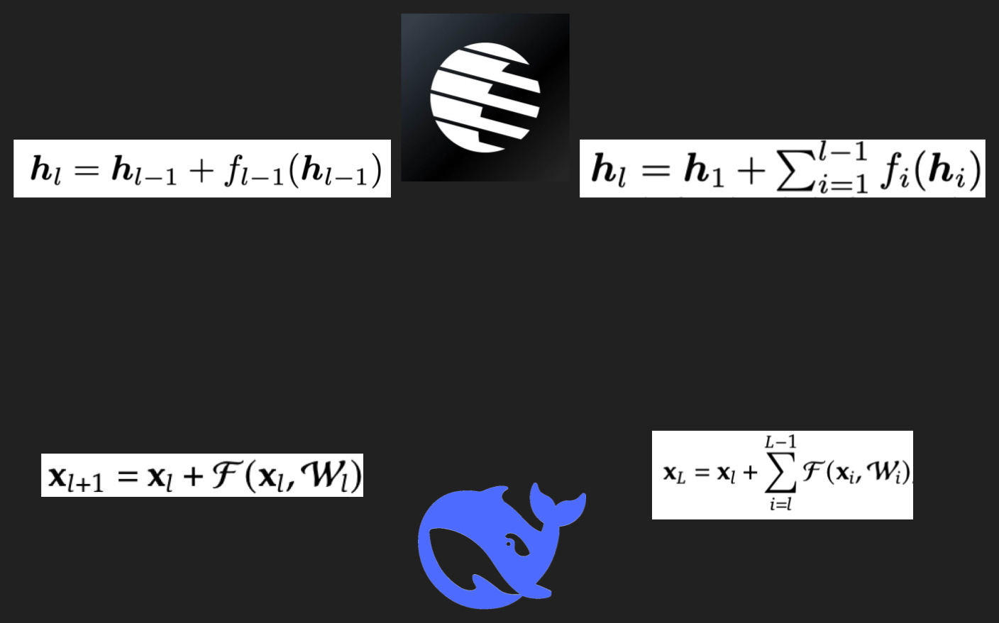
I also need to introduce the DeepSeek versions of these equations, on the bottom row. They are mathematically identical, it’s just that the DeepSeek version includes the weights W of the attention or FFN that the Moonshot version omits.
What would our man Rich say about this?
Yes, more learning!
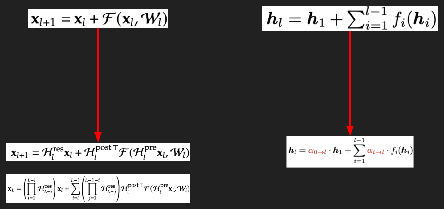
So let’s do more learning. Onto both of these equations we’re going to add new learnable parameters.
For DeepSeek on the left, it’s these matrices H, in three different varieties. We’ll see exactly what they are in a later slide, but for now just remember that the H matrices - “Hyper-Connections” in the jargon - are our new learnable parameters.
Note that the bottom equation, the even more fiendish-looking one, is the iterative version. So that’s directly comparable to iterative equation from Moonshot. I just didn’t want to make too big a leap at once.
Now for Moonshot on the right, the knob to turn is alpha, a single number rather than a matrix. That single number comes from some matrix math though, so I guess you could say we’ve abstracted the complexity away from this equation.
Anyway, the point is they’re both on to the same insight: the implicit equal weighting across all the layers for standard residuals is leaving something on the table.
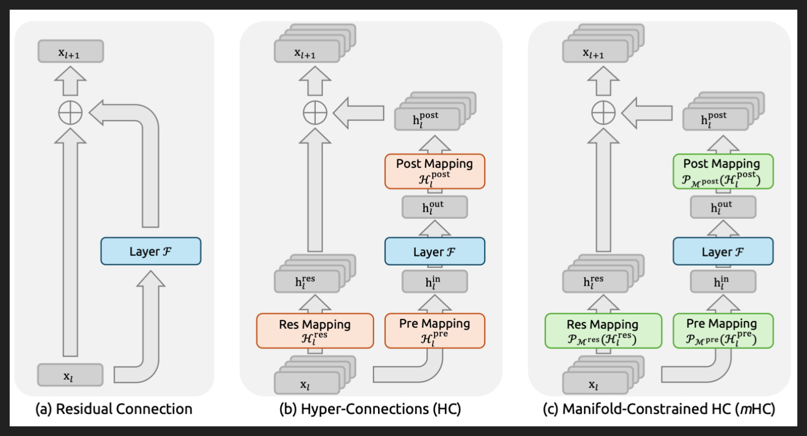
Now that we know how DeepSeek and Moonshot’s approaches are similar, we can precisely parse their differences.
Here’s a graphic from the mHC paper laying out their changes in two steps. We start with the standard residual connection, adding the original input of an attention or FFN layer to the output of that layer.
To go from connections to hyper-connections, we have to split the input into many different channels, many different parallel lanes, which is why they show some of the hidden states as multiple boxes now. Mathematically, we’re taking the vector x at the very start of the model and just copying it n times, so that x is now a matrix with n identical columns. But the columns are all gonna go on their own journey so to speak through their individual channels in the model, only to be collapsed back into a single vector all the way at the end of the model. So if we look at a random layer in the middle, the different channels are going to have different values of x_el.
Now we can get a little better sense of our H matrices. We have H^res for adjusting the original input, H^pre for adjusting the input before it goes to the attention or FFN layer, and H^post for adjusting the output of that layer. That’s three new knobs per layer, across all the layers. And the extra channels allow more information to flow as well.
So this Hyper-Connections part, the middle graphic, is actually not from DeepSeek - it’s from ByteDance, and the paper came out in September 2024. So what did DeepSeek contribute with their updated version in December 2025? And why didn’t anyone actually adopt Hyper-Connections in the 15 months between the two?
Well in addition to drawing attention to it with their respected scientific brand, DeepSeek pointed to a different component of the transformer for inspiration: the normalization layer.
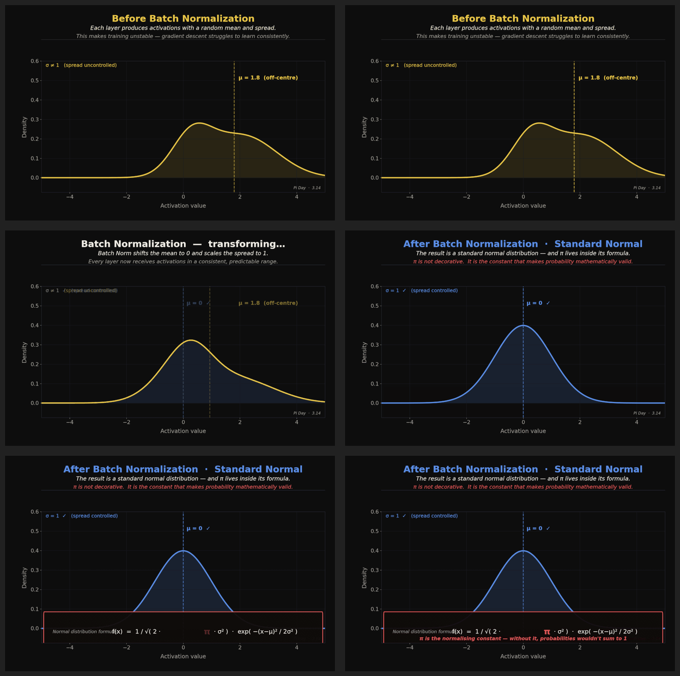
We haven’t talked much about normalization because it doesn’t really process information in the same way the attention and FFN layers do. It’s more of a preprocessing or post-processing step, to make the hidden state better suited for the next layer.
The basic idea is simple: if your layers are only trained for a certain shape or distribution of inputs, then you have to get your outputs back into that shape, or you risk unexpected behavior. Usually this shows up as failed training runs.
Normalization is a feature of all models, and even appears in the original Transformer paper. But you don’t need separate normalizers for residuals because the hidden states are already normalized!
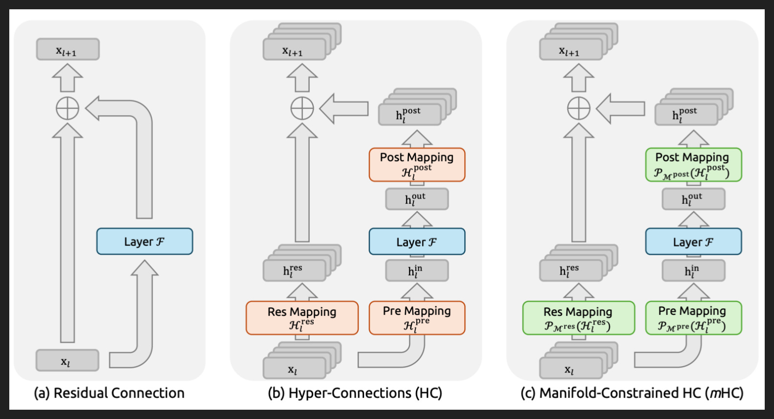
This is what the original Hyper-Connections authors neglected, that the DeepSeek team fixed.
On paper, all they did was add this normalizing function, abbreviated as P_M, to the H matrices.
In practice though, they did a ton of gnarly engineering to make it work at scale. In the end, their technique only increased the required compute about 7% on the 27B test model they trained, but it took a lot of cleverness to get there.
By the way, the “manifold-constrained” part of their technique is just a fancy way of saying the H matrices have to have all the rows sum to 1 and all the columns sum to 1. That range of potential matrix values forms the “manifold” that the H matrices live on. It’s like the unit circle, which contains all the x and y points where the radius is 1, but in way more dimensions.
So that’s mHC: more channels, and a stability trick to make it actually work.
Now let’s look at Attention Residuals from Moonshot.
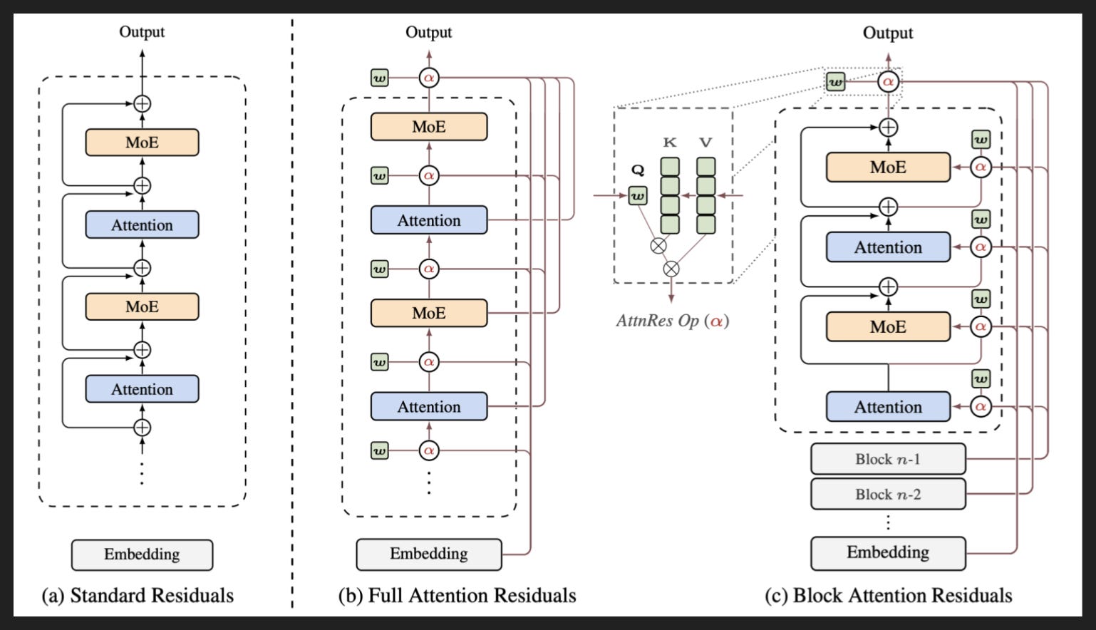
Next to our friend in image A, image B has two key changes.
First, instead of direct connections only between neighboring layers, there are direct connections between every layer. Like you can see the Embedding layer at the front touches all the attention and FFN layers, and then the first attention layer touches all the future layers, etc etc.
Second, there’s this alpha number instead of a plus sign. That’s our coefficient that tells us how much to pay attention to the residual. And if we look between images B and C, we see a diagram describing how alpha is calculated.
I’ll come back to that in a minute. Right now I quickly want to acknowledge image C, which is a version of image B but altered for scalability. We’re not going to get into it really, but just know that when you’re training a big model, you have to split up work between GPUs, and that causes problems with the normal attention residuals system.
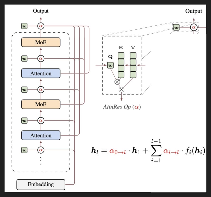
So, back to alpha. Again, that’s going to say how much each residual should factor in.
And each connection gets its own alpha. In the formula there we see the first one between layer zero and the current layer “el”, then alphas for each connection to “el”.
To calculate alpha, they’re going to use the oldest trick in the Transformer book: attention.
Remember, the job of attention is to decide what is important in the input when deciding on the output. And remember, we only predict one token at a time, so that outputted token becomes part of the input on the next go-around.
Mechanically, attention does this by taking the input and looking at it through three different lenses:
Query - the input as a question, as the thing that guides the output
Key - the input as the available information, as the stuff to possibly pay attention to. The query times the key tells you which connections between tokens are strongest, which other tokens to look at closely for any given input token
Value - what each token represents, what it actually means. Like a dictionary definition, but richer
That’s all standard stuff as a layer in the transformer, but what does it mean to use attention for residuals?
Well, two things. First, the query vector is actually NOT coming from the same place as the key and value vectors. It’s this vector w, which is specific to each layer even though it doesn’t have the subscript “el” in this diagram. This w vector learns how much of each prior hidden state to incorporate in the current hidden state.
Second, the key and value roles actually translate quite well. Each little green block there represents the hidden state from an earlier layer. In this case, we have the hidden state from the first four layers. So Q dot K is going to say how much of each hidden state we want to incorporate - that’s alpha - and then that times V is going to provide the actual information from the hidden state.
So we’ve taken the attention mechanism and turned it 90 degrees so to speak, looking at relations between layers instead of relations between inputs. We just had to be a little bit clever about the queries.
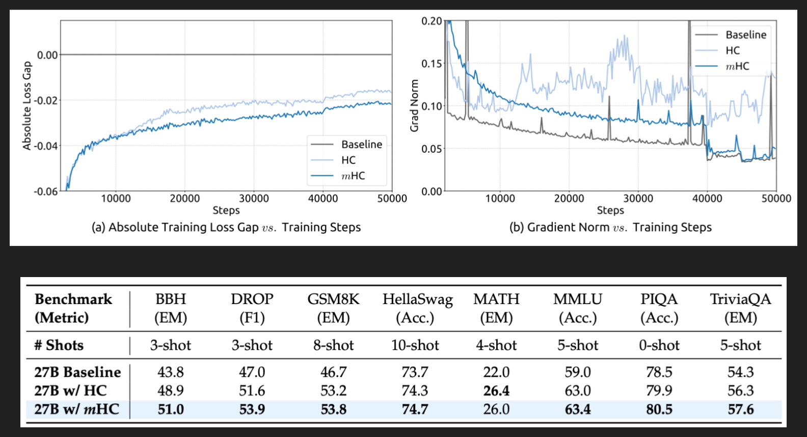
Now frankly it’s going to be challenging to compare the results of these two methods. Even though they work on the same part of the model, they tested by training two completely different models in terms of size, architecture, and data. So let’s start out with individual results.
For mHC, they picked two metrics: quality and stability.
For quality, they show it two ways:
Top left, there’s a graph of the relative difference in loss during training. Negative numbers mean the loss was relatively lower than baseline. So we see here that both HC techniques work, although mHC works better
Bottom, there’s a table of where their chosen benchmarks landed at the end of training. It’s a fine range of benchmarks, covering language ability, commonsense reasoning, math, STEM, code, and question-answering
From those two mHC appears to have a tiny, possibly insignificant edge over HC.
But then you take a look at the top right, which is a proxy for stability. The thing on the y axis, “gradient norm”, is basically a measure of update size. What you’d like to see is a smooth, gentle downward curve, bottoming out just as you stop training. In practice you always have some spikes, but the overall trend should look like the baseline in grey.
And you do get that with mHC. But you don’t get that with just HC, because HC doesn’t normalize to that manifold we discussed earlier. So you’re risking instability here, like wasted cycles or even wasted whole pretraining runs. For a toy model that’s fine, but when each pretraining run costs millions of dollars, you cannot afford instability like that.
So the story of mHC seems to be: 7% more overhead, for a little better quality at no risk. Probably a good trade.
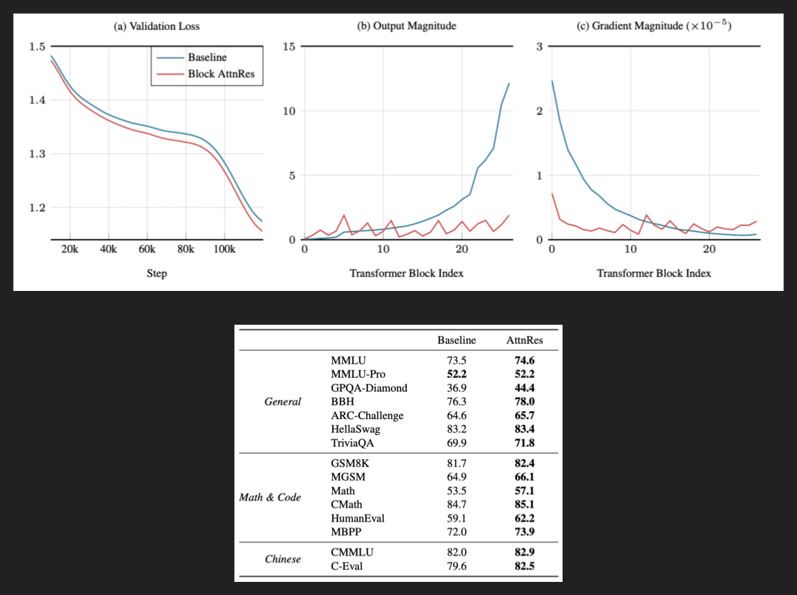
The Moonshot folks have gone for something similar here. We’re looking at absolute loss instead of relative, there in the top left, and we have a wider array of benchmarks. But it’s the same story: a modest increase in quality across the board.
And on the stability side, we get two graphs from training: the size out the outputs per layer in the middle, and the size of the changes from training (aka the gradient) per layer.
For the middle graph, what you normally see is that later layers have to use bigger numbers, since normally the residuals keep adding to each other. Bigger numbers risk instability, or loss of signal depending on how you look at it.
For the right graph, it’s the same story but backwards; the initial layers in a standard transformer have to make huge changes in order to impact the final layer.
But with AttnRes, in both cases you’re pretty flat in magnitude.
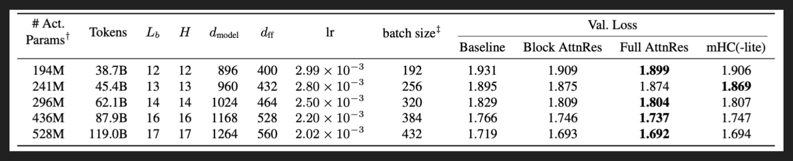
Luckily for us, the Moonshot paper does compare directly to mHC in one table.
It looks at models of increasing size, with other aspects like training data growing in proportion. And it seems here that AttnRes is on par with mHC, even when you have to make engineering compromises as Block AttnRes does.
So to me it seems the simpler method, AttnRes, is the winner. But it also makes me wonder if there aren’t other solutions at work in the closed labs.
My Takeaways
Moonshot may have bested DeepSeek here
Not exactly fair though, given mHC came out before AttnRes
But also, mHC is a change on top of HC, so perhaps a smaller contribution
AttnRes is more elegant
But mHC is more impressive - the math they pulled out to get the H matrices constrained to that manifold is arcane
Perhaps Moonshot will break into the S-tier with Qwen and DeepSeek
I doubt DeepSeek will regress to A-tier