


Originally presented as a live talk on October 21, 2026

Background

Since this is a paper about the mechanics of RL, I wanted to start with a low-level tour through modern-day RL.
RL is a form of model training. Training means changing the parameters of the model so that it performs better. The parameters are basically the weights in our embedding, attention, and feed-forward matrices, although technically there are other parameters.
So how do we take a model-level result - whether or not a response was good and thus rewarded - into all these individual changes to parameters?
Let’s work backwards from the end: the changes to parameters.
To change the parameter, which is really just a number, we need to know how much to change that number by. We take the existing number, θ (theta), and subtract from it the amount we want it to change. That amount has two components: the learning rate, η (eta); and the gradient, g. The learning rate is a hyperparameter you set manually during training. The gradient, however, comes from your loss.

This is the part where we go from individual parameters to the entire model. When you use a model, mostly what you’re doing is a bunch of matrix multiplications, with a few other mathematical operations thrown in. That chain of calculations is how we can trace the influence of each parameter on the final output. Sometimes people call this chain the “forward pass”.
Which implies the existence of a “backward pass” right? Indeed there is one, and it’s where information from training gets disbursed to all the individual parameters. But we need some information to pass backward, something based on the final output.
That information is the loss. I’m going to punt on where the loss comes from right now, so just think of it as a way to give a specific number or score to each token in a response. The lower the loss, the better the token is.
So we have our loss, and we have the chain of calculations that led to the tokens that produced the loss. On the backward pass, we use the chain rule from calculus to see how much a change in each parameter, each link in our chain of calculations, impacts the loss. In calculus terms, we take the gradient of the loss with respect to the parameters, which is what we have written here.
So we have our forward pass to generate responses, then somehow we calculate loss, then we use the loss to calculate gradients, which we then use to update parameters. What is that missing piece in the middle?
As you’d expect, it takes in responses and outputs loss. And how exactly you get from one to the other is where a lot of training algorithm magic lies. PPO, DPO, GRPO, DAPO - these RL training algorithms are all about collecting responses and turning them into loss.
Today’s paper is about GRPO, which stands for Group Relative Policy Optimization. Let’s see how GRPO turns responses into loss.
First, we need responses. Specifically, we’re going to get K responses per prompt. How big or small to make the group is an important part of today’s paper, so keep that K in mind.
Next, we’re going to score our K responses. Often we use GRPO with RLVR, meaning there is one verifiable, ground-truth answer. Usually the response earns a reward of 1 for a correct response and a reward of 0 for anything else. Rubrics also work with GRPO, since they can also numerically score and reward every response in a group, but today’s paper does RLVR.
That process of generating and scoring K responses is likely already familiar to you if you’ve worked with RLVR data. In fact, the other terms familiar to data folks - rubrics, RLHF, RL environments - also cover the same ground between the prompt and the rewards. However, there are more steps to go to reach our loss. These next steps are where the different algorithms play. That means GRPO and its variants like DAPO, but it also means classic algorithms like PPO and REINFORCE (yes, it’s an acronym).
Broadly speaking, the next step is to turn rewards into advantages, which are like rewards but transformed or altered according to the specifics of the algorithm.
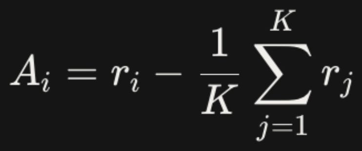
For GRPO, our advantages depend on how well a response did relative to the rest of its group, hence the name Group Relative Policy Optimization. Specifically, we’re going to subtract the average reward from each response’s reward. In classic GRPO we also divide the result by the standard deviation of the group’s rewards, but today’s paper drops that part.
I have the advantage formula right here. For response i, the advantage is the reward minus the average of all rewards amongst the K responses.
Let me give a concrete numerical example. Say we have K=4 responses, with 3 incorrect responses and 1 correct response. Our reward is binary, so that means the reward for the incorrect responses is 0 and the reward for the correct response is 1.
The average reward is thus 1/4, i.e. 0.25. So the advantage for the incorrect responses is 0 - 0.25 = -0.25, and the advantage for the correct response is 1 - 0.25 = 0.75.
All well and good, but what is the purpose of this mutation from reward to advantage? To see the benefit, let’s examine a few cases.
In a mixed case like we just saw, the incorrect responses now have a negative advantage, not just a nil reward. We’re actively punishing the incorrect responses rather than just leaving them out.
Now, what if all the responses are correct? The rewards are all 1, but it seems there’s nothing for the model to learn. Why should we spend time and compute training when the model is already perfect here?
Advantages take care of the problem for us. Since the average reward is 1, then the advantage for each response is 1 - 1 = 0. No advantage, no learning. Same deal with all incorrect responses, although given the rewards are all zero it’s no surprise there’s no learning to be done.
For this paper, we should also consider what happens with much larger K and an extreme ratio of correct to incorrect - either a single correct answer with the rest incorrect, or a single incorrect answer with the rest correct.
For the first case, the average reward will be close to 0, since almost all the responses are incorrect. The advantage for the one correct response will be close to 1, and for the rest it will be close to 0.
For the second case, the average reward will be close to 1, since almost all the responses are correct. The advantage for the one incorrect response will be close to -1, and for the rest it will be close to 0.

Now that we have an advantage for each response in a group, we need one other quantity: the importance ratio, often just called “importance”.
But to even understand what the importance is, we first have to understand a bit about the mechanics of RL.
Earlier, when I described how GRPO gets a group of responses and scores them and turns them into advantages, I glossed over exactly where the responses come from. If I handwave and just say “the model”, it’s not exactly wrong, but it doesn’t address which version of the model the responses came from.
Remember, the end result of this big journey from initial input to final weight change is a new version of the model. During RL, we make many incremental changes to our model, many updates, which means the responses from “the model” are really responses from a model - a single, short-lived model we soon update again.
Over the course of training then, you accrue many responses per prompt, per update. Not every prompt runs on every update, but most prompts will run on more than one update.
In training, responses that came from the exact same version of the model you are about to update are called “on-policy”. Responses that came from older versions are called “off-policy”. Technically any response that isn’t on-policy is off-policy, so like a response from a completely different model is also off-policy.
Exactly how “off” we are depends on how many updates ago we generated the response. Usually it’s okay to train with responses that are a little off-policy, but past a certain point they can be harmful. Sometimes people call this split “fresh” vs “stale”. So on-policy data is always fresh, some barely off-policy data may also be fresh, then the rest is stale. There is no universal rule dividing fresh from stale; as we’ll see in the paper, it’s an empirical matter.
Now within our off-policy but still fresh data, we need a measurement of the difference between the old policy that generated the data and the current policy that we’re updating. The way we measure is per token. Specifically, for the chosen token at a position, we measure the likelihood of that token on both policies. The importance is simply the ratio of the likelihood from the current policy to the likelihood from the old policy.
Here is our importance formula. For response i and token t, the importance equals the likelihood of the current token from the current model π_θ given the prompt x and all the prior tokens in the response y, divided by the likelihood of the current token from the older model that generated the response π_θ_old, again given the prompt x and all the prior tokens in the response y.
The importance is the mathematical reason why off-policy data can be so dangerous. In the extreme case, like using a completely different model to generate responses, one likelihood can be close to 1 and another can be close to 0. 0/1 = 0, and 1/0 approaches infinity, so variance in importance is enormous. The resulting variance in loss per token can cause inappropriately small or large updates.
Of course if your data is on-policy, then both policies are the same, so your importance is always 1. It slows down training too much to get all your data on-policy, so that balance between safety and speed is important.

With importance and advantage, we pretty much have what we need to compose the GRPO loss.
For completeness, I’ll note what we left out, reading from left to right:
The expected value operator E, which basically means we’re averaging the loss over all the prompts in our batch
The 1/|y_i|, again a sort of averaging, this time over all the tokens t in the response y_i. Often not used in GRPO
The min and clip, which means that we cut off the importance if it’s too far above or below 1, in this case by the amount ϵ
These aspects are not specific to GRPO and thus are not important background for today’s paper. I also left out KL divergence, another sort of safeguard against extreme updates that appears in many loss formulas, because in this paper they don’t use it.
Now that we have the mechanics of GRPO down, let’s talk about what it means for RLVR.
When we discussed advantages before, we saw that prompts are too easy or too hard for a model if every response has advantage zero, i.e. all the answers are correct or all the answers are incorrect.
As we know though, model capabilities are always advancing, so over time the balance isn’t really symmetrical; it’s always bad to generate prompts that are too easy, but at some point the prompts that are currently too hard no longer will be. Similarly, the prompts that are almost too easy now will become too easy soon, whether during the current training run, or after the next big pretrain, or from the next architecture change, etc etc. That means the long-term value is always weighted towards harder tasks. So the trick is to have a hard floor on difficulty, but a soft ceiling.
One common way to assess difficulty is to give a model some number of chances to produce a correct answer. The term for this is “pass@k”. For a given dataset, pass@k is the share of tasks the model correctly solves within k tries. And yes, that is a second “k” number to keep track of, alongside the k responses we ask for during GRPO. I don’t make the terminology, don’t shoot the messenger!
Anyway, when researchers measure difficulty, usually they pick a small value for k, like 1 or 3 or 8. The idea is to keep the number of attempts reasonable, like within what a user would actually put up with when asking the model to try again.
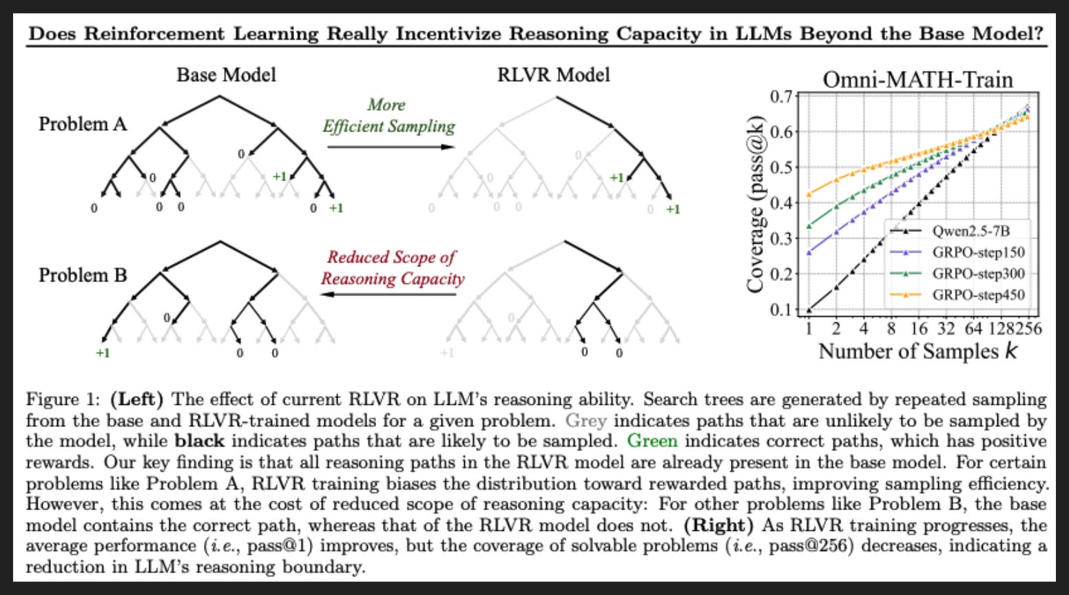
However, some researchers whack k up to a really high number, like 256, to see if the model in question can possibly solve the problem. That’s a different, more theoretical question, and it has produced some interesting work. I’ve covered a couple such papers before, including the one shown here. The researchers found that a base model with no post-training at all can eventually produce pretty much any answer a post-trained version can, if you use a high enough k. It’s good evidence of elicitation: RL brings forth what was already in the model, rather than teaching something new.
To be clear, RL is still valuable, since for users it’s important to receive the right response on the first try most of the time. But for today’s paper, keep in mind how important it is to dial up the number of attempts in order to finally receive a correct response. If the right answer is in there somewhere, it’s worth finding.
The Paper
On the last slide, we looked at dialing up the number of responses in eval. What about in training?
Well as you’d expect from the last slide, if you give the model more chances, it is more likely to produce a correct response. And if you have at least one correct response in your sea of incorrect responses, you have at least some advantage to put in your loss function.
So why not just whack up K, the number of responses per prompt in GRPO? Surely it will help to turn these hard prompts into training signal.
Well sometimes people do that. And this paper is about how to do that better.
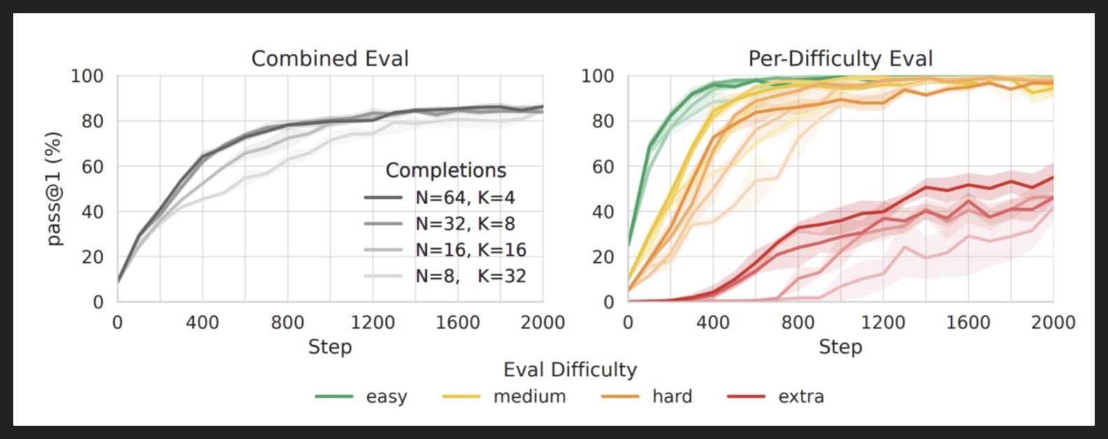
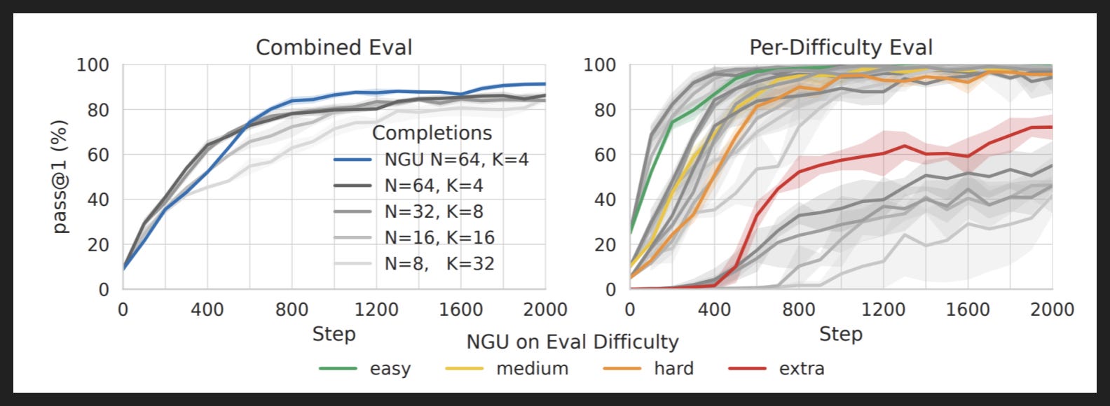
The graphs above show the existing situation, using various RL settings on Qwen2.5 0.5B Instruct, evaluated on a math benchmark called GSM8k. For a fixed compute budget, minus differences in response length, you have to decrease the number of prompts if you want to increase the number of responses per prompt. That’s the Completions table, where N is the number of prompts and K is the number of responses. The left graph tells us that actually, fewer responses on more prompts is better.
But the real story is on the right: increasing K actually hurts performance on the hardest problems the most! Not only that, it hurts performance on some less hard problems too. What is going on?
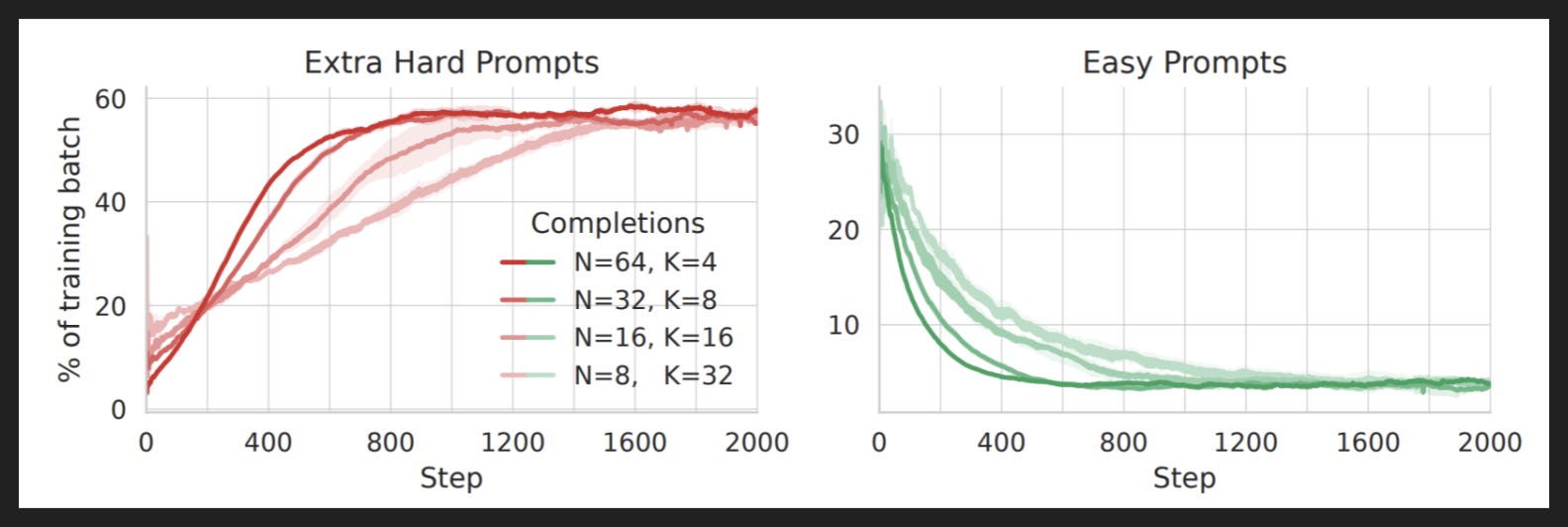
It’s two things really. For one, it’s a waste of compute to get 32 responses to an easy problem. If you leave K at 4, you quickly and cheaply find the easy problems where all 4 responses are correct, drop them from the training set, and bring in new prompts that may have some learning juice in them. So small K means more rapidly reallocating fixed compute budget to harder problems.
For another, requesting more responses for the same easy prompt risks receiving a wrong answer! It is the inverse, but far less appreciated, version of what we talked about for hard prompts. With just one incorrect response, now your easy prompt goes from quickly dropped to retained, thus using more precious compute going forward, and altering the weights. Given the inherent risk of changing weights and low signal-to-noise ratio here, training on easy prompts due to fluke poor responses is not a good idea.
So on the one hand we need large K in order to find rare solutions to hard, valuable prompts. But on the other hand, increasing K wastes compute and risks regression. What are we to do?
The answer is to do both. Or rather, to adjust K depending on the prompt, rather than setting one K universally.
Start with K=4 across the board. That’s the cheap first pass, and it knocks out any prompts that are already too easy. It also gets nonzero advantages on many other prompts, where some but not all of the responses are correct. So far, it’s standard GRPO.
The trick comes for the hard prompts, where none of the 4 responses are correct. Instead of dropping them, we never give up (NGU), and keep increasing K until we get a correct response. Once we get a correct response, we stop generation for that prompt and start training.
Now it’s actually not quite never; they do introduce a small chance of giving up, like 5% here and slightly higher in other experiments, on each increase of K. Some problems really will be out of reach for a model, especially the small models they tested here, so trying forever will be a waste of compute. But the point is that NGU dynamically allocates compute to the hardest problems.
And the results are promising. The lines to compare are the blue + darkest grey on the left, and the colored + darkest grey on the right. For the same number of prompts and initial number of responses, NGU helps a bit overall, but especially helps on the hardest problems - the ones where the initial model wasn’t getting any correct responses at all in an initial test run of 1,024 responses per prompt.
That’s exactly what we hope to get out of RL. In standard RL, what we actually get is saturation on the easiest prompts and barely any movement on the hardest prompts. Like we saw last slide, standard RLVR can totally misallocate resources. The researchers call this “the Matthew Effect in RL for LLMs”, named after the original Matthew Effect from sociology, which basically says that people accrue success in proportion to their existing success. In economics, the quick encapsulation is “the rich get richer”; in RL, it’s “the successful problems get more successful”.
NGU fixes that.
Now as we discussed in the background slides, RL training happens in many steps, and sometimes the copy of the model that’s producing responses lags the copy of the model that’s receiving updates to its parameters.
With a fixed K, you can keep that drift between models small. However, with NGU, K is variable per prompt. As a result, the responses can become quite stale, with the generator model several update steps behind the trained model.
We know from earlier there is a balance between safety and efficiency, between how fresh we need our responses to be and how few times we can get away with replacing the generator model with the latest copy. However, there is an additional wrinkle with NGU.
Let’s say it takes 256 attempts until one response is finally correct. On the one hand, most of the 256 responses are probably stale by now, so we shouldn’t use them in training. But on the other hand, it’s really important information that it took 256 tries to finally get something right! How can we keep that difficulty information without risking bad behavior in training? How do we balance out the positive impact on advantages with the negative impact on importance ratios?
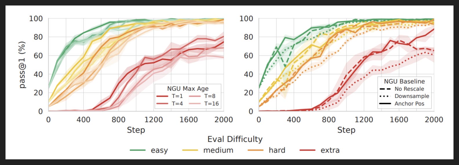
Well first, the researchers find that four update steps is the right cutoff, as shown on the left plot. Any response from a model up to four versions out of date is fresh enough to use still.
Second, the researchers use some simple but insightful math to rebalance the advantages.
Let’s continue with my example: 256 attempts, only one correct response. Assuming binary rewards, the advantage for the one correct response is 0.996, and the advantage for each incorrect response is -0.0039. So the advantages are basically binary too.
Let’s now say that all but 4 of the 256 attempts are stale. If we naively threw them all out, the advantage for the one correct response would be 0.75, and the advantage for each incorrect response would be -0.25. That’s a major reduction in signal for the correct response, although a nice bump up in the penalty for incorrect responses.
Now let’s take the best of both worlds: keep the original advantage of the one correct response, and adjust the advantage of the three remaining negative responses to match. So that’s 0.996 still for the correct response, and now -0.332 for each negative response. We now have strong signal in both directions.
The researchers call their approach “anchoring”, and the plot on the right shows how it improves outcomes relative to the naive approach and to one other approach called “downsampling”.

So far we’ve been looking at performance on math, which is a super common domain for training and evaluating LLMs on.
To ensure NGU is robust, the researchers test it on a different domain: programming, but in the form of puzzles. Specifically, the benchmark has the model play the game Manufactoria, where the player creates robot factories that process sequences of colored tape. It might sound completely strange, but it’s actually a somewhat literal construction of a Turing machine, which is the simplest conceptual thing you can program. So it’s programming, which is very in-distribution, but in a very out-of-distribution setting.
What the researchers find is the model needs some time to adapt to the game, to learn the harness before it can really learn how to succeed. If you try to tag difficulty early on, you get bad intel about which prompts are easy and hard. The Matthew Effect seems to disappear.
However, if you wait for the model to adapt to the harness, then bucket by difficulty, it works just fine. In this case, it only took about 100 RL steps, which is a small fraction of the 3k step budget.
It’s not a crucial part of NGU per se in my view, but it’s a nice example in the wild of how the relationship between model and harness is a two-way street.

Continuing with the Manufactoria benchmark, we see some familiar patterns in different forms.
First, a quick word about how to measure success on programming benchmarks. Usually each problem has a set of tests, rather than the one final answer from math. There are two ways to report on the test set: as a percent of tests that passed, and as a binary on whether the entire set passed or not. Here they call the first approach “combined tests” and the second approach “all-tests”.
Anyway, we see on the left that NGU helps pass more tests across all problems. In the middle, we see in particular that hard tests get the most help, which is where most of the opportunity was anyway. Great alignment of compute with need, as expected with NGU.
We also see a big jump in all-tests, i.e. in problems with totally complete solutions. In fact, plain GRPO passes all tests on zero problems! That’s arguably more important, since we expect our coding agents to build to spec and not just close to spec. It’s the same reason ProgramBench reports all-tests as the top-line metric rather than combined tests.
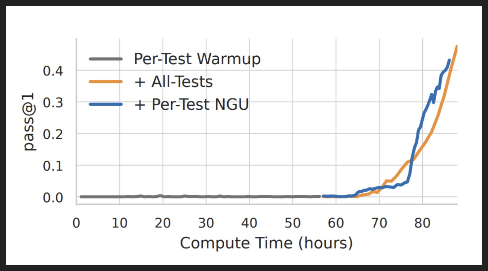
There’s actually some prior art on training to solve Manufactoria. In it, the researchers first gave per-test rewards, watched until performance plateaued, and then switched to all-test rewards. You can’t do all-tests to start because none of the responses will be correct, so you can’t start learning.
NGU avoids this one-two step. As the chart shows, simply adding NGU to per-test rewards pretty much matches all-tests, even when you add NGU to an existing checkpoint that has undergone significant RL without it, as they did here. Again, NGU naturally addresses issues other methods must specifically design for.
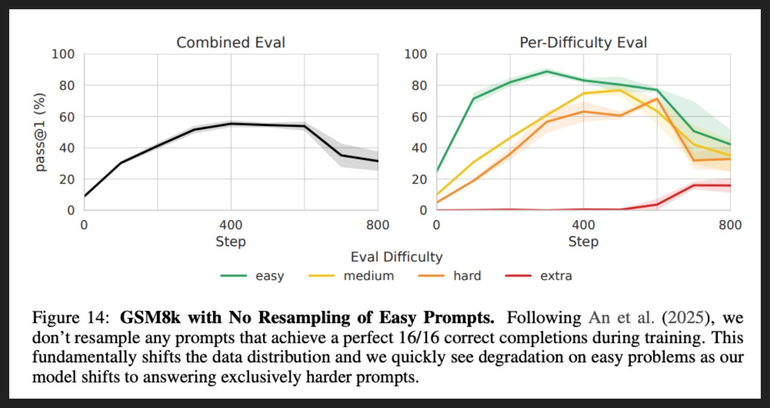
Finally, one note about easy prompts. I mentioned earlier that easy prompts leave the training set, replaced by other prompts that may still have something to teach the model, so compute can focus on the harder prompts.
However, additional training does not guarantee improved performance, and sometimes gains in one place cause losses elsewhere. In other words, models can regress in areas we’re not watching.
The chart here shows how that looks. While performance improves for a while, eventually it degrades, roughly in proportion to how much was dropped from a difficulty bucket.
The simplest fix is to never drop examples, which costs compute of course but is kind of like paying insurance on the gains you’ve made.
But the researchers think we can do better. They propose dropping temporarily, after each batch, and then bringing back the prompts at the start of the next batch. Since NGU allows K to start small and grow on hard problems as needed, it’s cheap to re-check supposedly easy prompts at the start of each batch. As a bonus, their method lets regressions show up naturally and early, rather than as nasty surprises during eval.
My Takeaways
Clean insights that everyone should adopt
Never give up
Never risk fluke wrong answers on easy examples
Never permanently drop easy examples
Data that may seem too hard can still be valuable
If we never give up, eventually it won’t be too hard
But if all data is too hard, you can’t start learning. Training data needs distributions
Maybe there is a way to more quickly elicit correct responses
Or to elicit them at all, if even at huge K the model produces none
The former is about saving valuable compute; the latter is about saving valuable training data