


Originally presented as a live talk on September 16, 2026

Background
Let’s start with the company behind the model: Moonshot AI.
Moonshot AI was founded in China in March 2023, 50 years after the release of Pink Floyd’s The Dark Side of the Moon, after which the company is named. For context on AI progress at the time, ChatGPT came out in November 2022. Coincidentally, GPT-4, Claude 1, and Google Bard also came out in March 2023. So a pretty busy time! I remember hearing about new models from tons of new and no-name shops in 2023 and 2024, when models were still small enough for startups and even academic labs to pretrain on their own. Now of course there are few organizations worth tracking and everyone knows who they are.
Anyway, in October 2023 the first version of Kimi came out, as a chatbot for the Chinese market. Kimi K1.5 came out in January 2025 with the same approach, not making much fanfare from what I recall.
It wasn’t until the release of Kimi K2 in July 2025 that folks here really started paying attention to Moonshot. That’s because Kimi K2 was open weights, and those weights were huge: 1T parameters, the biggest open-weights model ever released at the time. Successive releases in the K2 series - K2.5, K2.6, K2.7 - held onto that record. DeepSeek took it with their V4 Pro release in April 2026, but Kimi K3 actually took it back again for Moonshot, with its incredible 2.8T total parameters.
Publicly releasing such a big model made Moonshot the perfect partner for AI startups that had decent access to compute but not nearly enough of it to pretrain their own models from scratch. So for example, Cursor’s Composer 2 used Kimi K2.5 as the base model and then post-trained for coding and use within Cursor, like with Cursor as the harness. More recently, Harvey’s Tenet did the same thing with Kimi K3 for long-horizon legal work.
Further increasing Moonshot AI’s status is their scientific work, which has improved in taste and impact as they have grown. We’ll touch on two particular topics a bit later when we do the technical side of background.
On the flip side though, we have heard repeated allegations of Moonshot distilling outputs from more advanced models to improve Kimi. Most recently, Anthropic claimed that Moonshot was even serving Claude instead of Kimi, using over 5k fake accounts in Singapore and Japan, so users of Moonshot’s APIs and chat tools were sometimes talking to Claude but told it was Kimi. There is some genuine debate about the merits of distillation, but there’s really no defense about selling someone else’s product as your own.
Still, the weights to Kimi K3 are out there and available on plenty of other inference providers, so we know it’s not all smoke and mirrors. My personal hunch is it’s more of an economic or GPU-related tactic than trying to cover for poor quality or something.
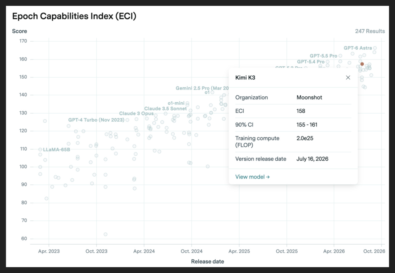
Speaking of Kimi K3 versus other models, here’s my go-to resource for checking model rankings and progress: the Epoch Capabilities Index (ECI), a composite of 50 benchmarks from several sources. The score on the y axis is supposed to reflect ranking relative to GPT-5, which definitionally scores 150.
ECI is a product of Epoch AI, a well established, independent research organization. I’d put them in the same bucket and tier as METR, whose famous time horizons graph we touch upon so often in Friendly Paper Review.
And in fact the trend is the same here as on the METR graph: a steady, unrelenting line of progress. It’s pretty remarkable how predictable frontier progress on ECI is.
As you can see from the displayed names, it’s always US labs in the lead. Mostly it’s OpenAI or Anthropic, although I spy Gemini on there. The sole red dot, off the frontier line, is Kimi K3.
There are really two ways to situate any model not on the frontier: the gap against the best current model, and the time lag since the first time a model reached the subject model’s score.
So if you look at other models available on the Kimi K3 release date of July 16th, Fable 5 was the best, with an ECI of 163. That’s five points ahead of Kimi K3, at 158. But what does that actually mean? It’s a bit abstract on its own.
That’s where the time lag helps. If you look left of the red dot, the first model to reach or exceed 158 was GPT-5.4 Pro, at 159. (GPT-5.4 scored 157.) That’s four, maybe four and a half months before Kimi K3 came out. So if you’re used to using only the best models, then you’re travelling back in time a third of a year when you use the latest Kimi.
In fact, the rough heuristic is that Chinese frontier models are about six months behind American frontier models. People freaked out at the time of the Kimi K3 release because on some measures it was on par with the leading US models, but with a little distance I think we’ve seen the time lag implied by the ECI score bear out - there was no mass exodus from Fable to Kimi because Fable was clearly better.
A couple other data points from this graph on recent models. First, Kimi K3 scores just above GPT-5.6 Luna and just below GPT-5.6 Terra. But Kimi is 50% more expensive than Terra and over 10x more expensive than Luna, which means it’s a poor economic choice on this basis but also implies it is larger than both models. So again, the leading US labs are ahead.
On the flip side though, Kimi K3 comes in slightly ahead of GLM-5.3 and Qwen3.8 Max, its top Chinese competition as of writing.
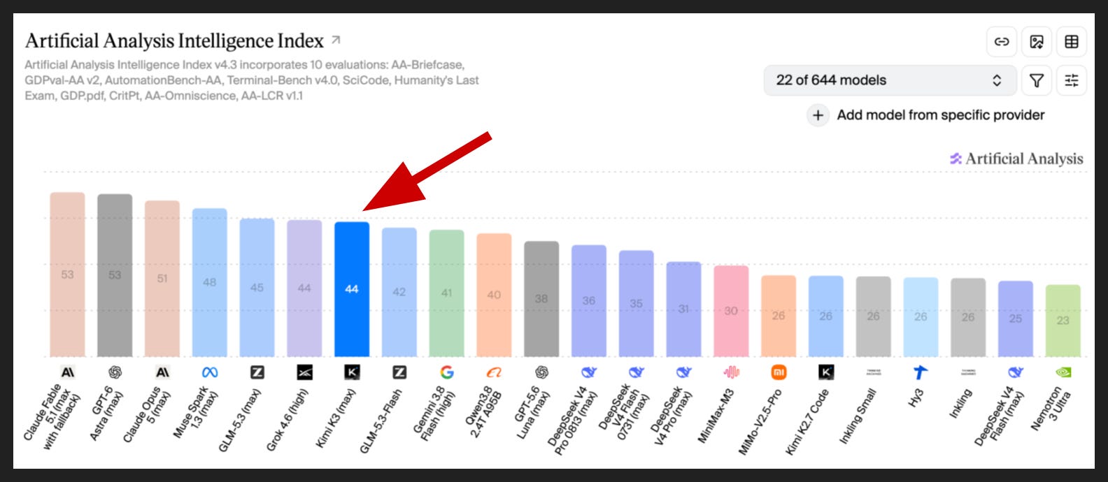
I will also throw Artificial Analysis out there as a decent source of information on model performance, although the index here only comprises 10 benchmarks. I like this chart because it’s easy to see where all the big players land.
So of course we have Anthropic and OpenAI at the top. Note that I have removed some of their models from the chart in the interest of visual clarity and variety, but they pretty much dominate the top slots.
Apparently Meta scores highly here, which impressed me, as does Grok 4.6, which is surely due to the good work of the Cursor folks who are now officially on board there. Kimi K3 trails just behind, virtually tied with GLM-5.3, another Chinese open-weights model that has made waves.
The biggest shock to me though is the cluster of DeepSeek bars spanning the 30s. DeepSeek is probably the most well respected Chinese lab, so it’s tough to see them lagging so badly. I’ll have more to say about them at next week’s Friendly Paper Review when we cover their most recent release, DeepSeek V4.1 Flash.
Okay, now let’s touch on some technical background before we get into the paper. I want to mention two bits of Moonshot prior art: Kimi Delta Attention (KDA), and Attention Residuals (AttnRes).
Let’s start by refreshing ourselves on attention, which is the basis for both.
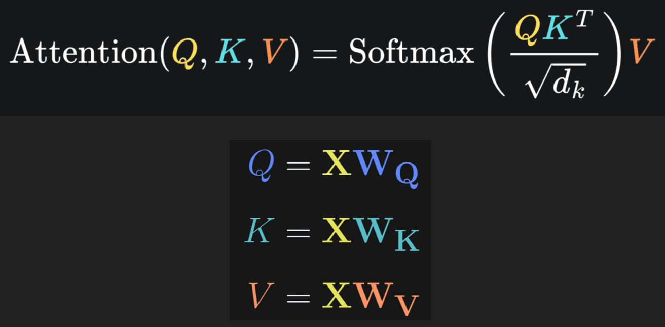
The purpose of attention is to figure out what stuff from the input X we need to take into account when predicting the next token. The way it does that is by looking at the input a few different ways: as queries (Q), keys (K), and values (V).
The query is the token in question, like the thing you’re going to compare other things to one at a time to determine the meaning of the pairing. Let’s say for example my query token is “red”.
The key is the other token, the one that’s going to modify the query and produce a pairing. Let’s say for example it’s “shoe”.
The query and the key combine to provide the attention score, which says how much we should care about that pairing. Don’t worry about the square root divisor and the softmax operator - those are just about keeping the numbers reasonable and bounded.
Finally, the value is the meaning of that pairing. “Red shoe” has one meaning, “blue shoe” would have another, and a nonsense combination like “red go” technically has a value but not a strong one.
By the way, the way you turn X into Q, K, and V is to multiply X by the relevant set of weights W. Those W matrices are what the model is really made of, plus the formulas that say how to use the matrices. The other parts of the model like the feed-forward network also have weights of course.
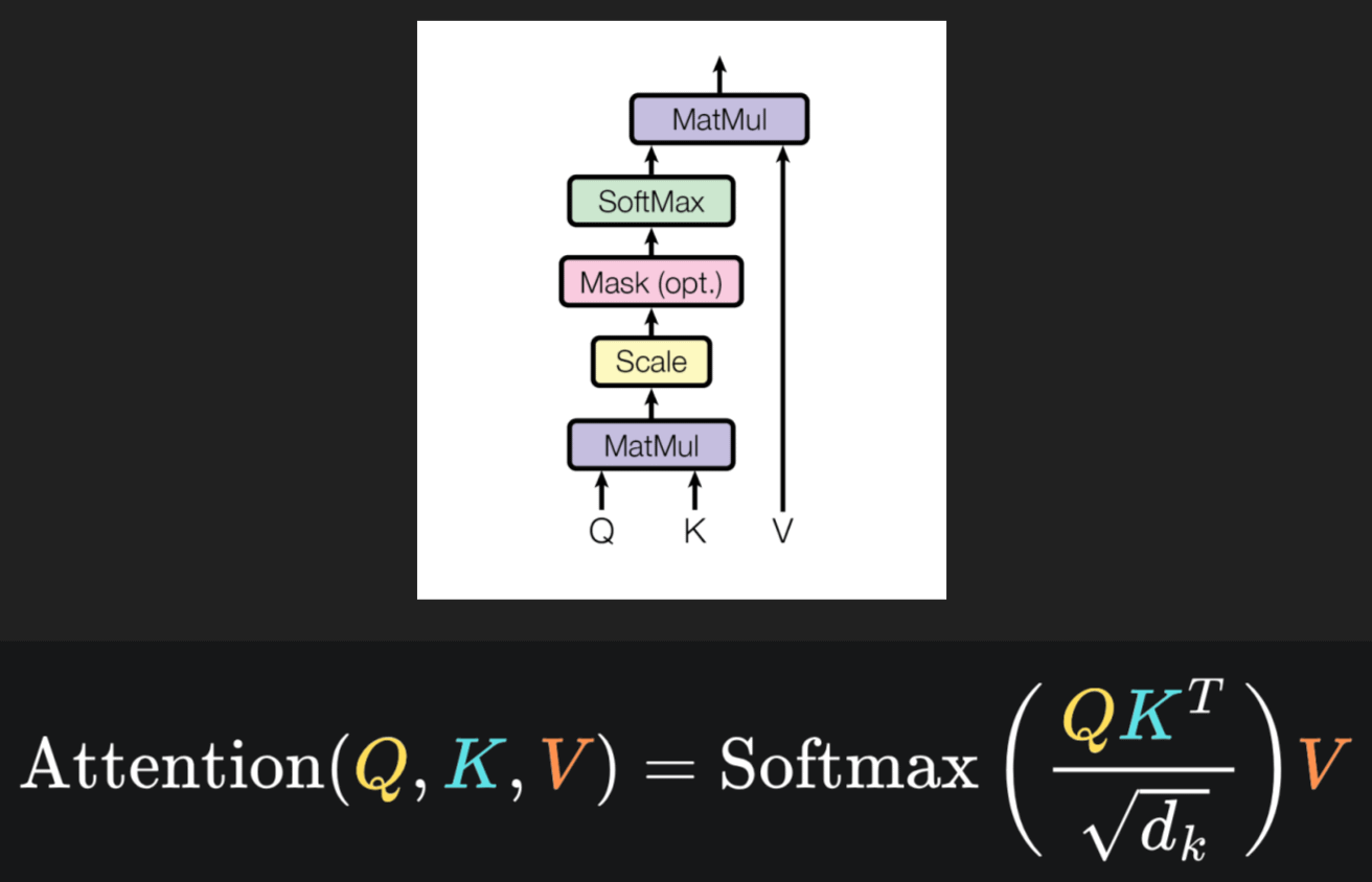
It has become conventional to present LLM architecture in diagrams, often like the one you see at the top here. Remember though, it is just math deep down - the diagram is equivalent to the formula we saw before, minus the pink “Mask” box which is optional. Keep this sort of diagram in mind for the next slide.
Now the biggest issue with the original attention formula is that it doesn’t scale well. By giving equal resources to every pairing of input tokens, the compute and memory loads grow as the size of that input squared. So-called “quadratic attention” is the highest quality variant, sure, but it’s often wasteful and certainly not practical in the agentic age where very long trajectories are the norm.
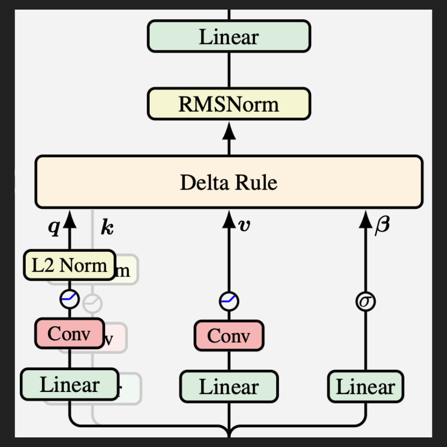
So instead of quadratic attention, where resource intensity grows as the square of the input size, people try various forms of linear attention, where intensity is directly proportional to input size.
And actually there’s a form of neural network that long predates attention and the whole transformer paradigm that already is linear in this way: the recurrent neural network (RNN).
I’m going to spare us the math and use an analogy instead. For quadratic attention, the model is keeping detailed notes and can go back and find anything. But for RNNs, the model gets a single page - a cheat sheet - that it can tweak and update as it processes more input. It’s lossy, but it’s much faster to review when thinking about what the next token should be.
But how to update that cheat sheet as each new token comes in?
That’s where the delta rule comes in. Again, putting the math aside, the basic version is to look at the difference between the predicted value and the actual value and update based on that difference, that delta. And the parameter beta, over on the right there, is a number between zero and one that controls how strongly to update based on the delta. For that reason, people call it the “learning rate”, although in the original paper they called it “writing strength”.
The graphic here shows DeltaNet, an RNN that incorporates the delta rule. Don’t worry about the elements we haven’t explicitly mentioned, like Linear and Conv and L2 norm.
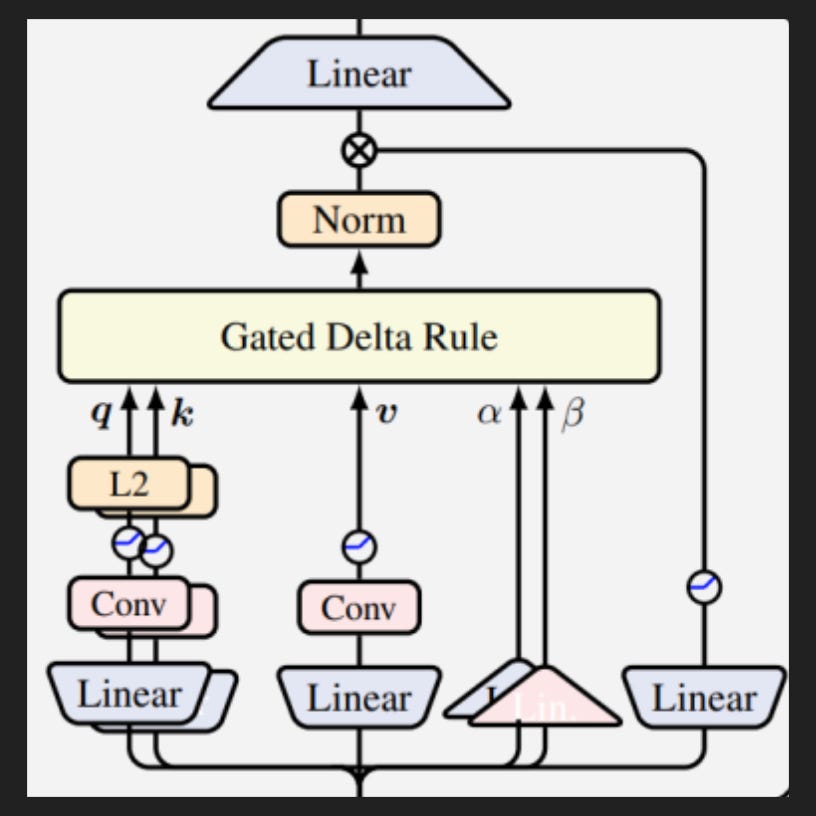
Now DeltaNet came out in mid 2024, and since then folks have settled on two key additions: a “forget gate”, alpha; and an “output gate”, the line on the right that goes around the delta rule and into that circle with an x. The gates give the design its name, Gated DeltaNet (GDN).
The forget gate alpha is basically the complementary knob to the learning rate beta, although they are independent. So let’s say you’ve got your cheat sheet, i.e. your recurrent state, and you process the next token.
If alpha and beta are both close to one, then you keep as much as possible from your cheat sheet but take great pains to record the information from that token. If the input is a really critical piece of the puzzle you’ve been assembling in your prior context, you could get that behavior.
If alpha and beta are both close to zero, then you write down nothing and you basically erase your cheat sheet. Maybe if your input clearly demonstrates the prior information is all outdated or irrelevant now yet no new information has come in, this would make sense.
If alpha is high but beta is low, then you’re keeping your cheat sheet as-is, like the current input is filler or repetitive etc.
Finally, if alpha is low but beta is high, then you’re clearing out space for the new stuff you’re taking in, really changing direction or maybe updating old stuff.
So that’s the forget gate. Then after your delta rule and a quick normalization for stability, the output gate decides how much of that layer’s output to keep as the information flows on to the next layer. Like if all that updating just wasn’t that important, the output gate can effectively toss it.
Overall the GDN is strictly superior to the regular ol’ DeltaNet in quality, which is why Moonshot picked it as the basis for KDA.
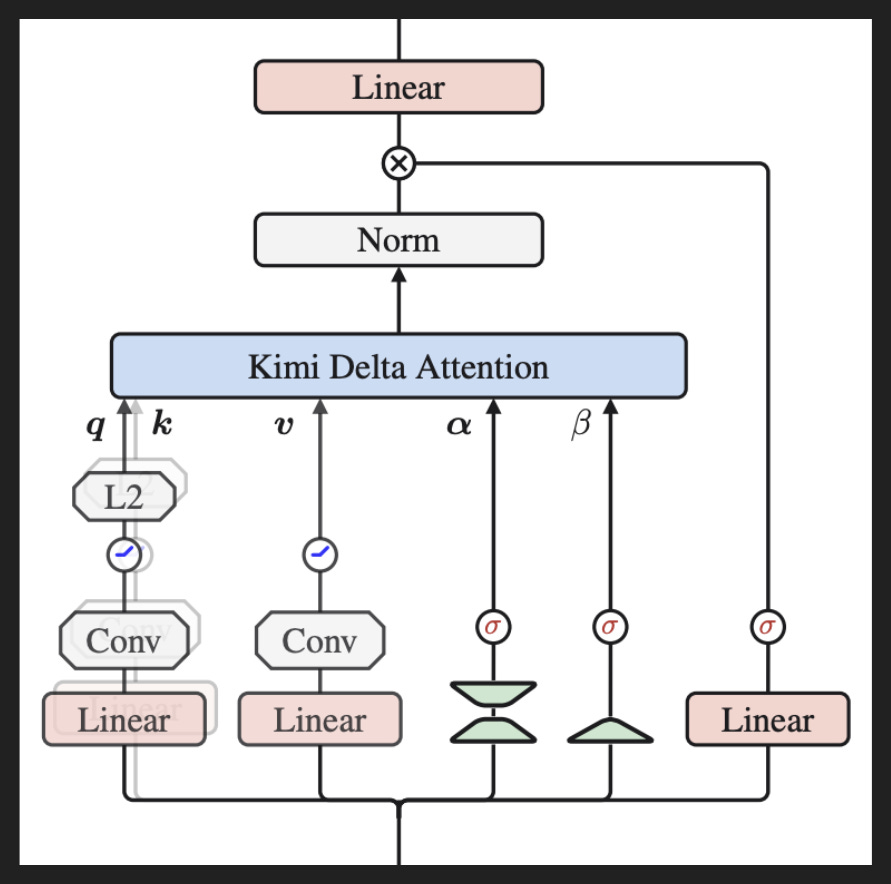
Speaking of which, here it is! Looks pretty similar right?
It’s subtle, but the main difference is that forget gate, alpha: it’s gone from a scalar to a vector. So now the forget gate can vary depending on more fine-grained aspects of the input.
Now there was a ton of gnarly engineering for KDA but also for GDN earlier to make all this new computation actually feasible, which we don’t need to get into here and isn’t visible with nice architecture diagrams like this. As is often the case, apparent simplicity often belies the real complexity.
So that is KDA in our pockets. Now to add AttnRes.
Luckily for us, I already did a Friendly Paper Review on this topic! And in another bit of happenstance, that FPR also covered a DeepSeek paper, just like we will be covering a DeepSeek model right after a Moonshot model. I guess when progress is this fast, you’re bound to get coincidences.
Because I already covered AttnRes in depth, I just want to quickly define a residual and how attention plays into it.
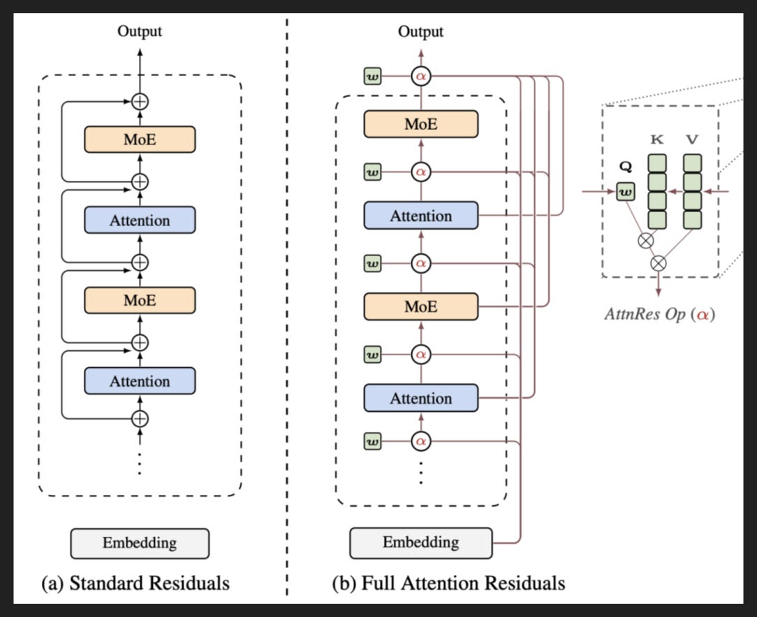
On the left we have a standard transformer diagram with embeddings to start, alternating layers of attention and feed-forward networks (in this case a mixture of experts [MoE]), and then output. They have neglected many details, but kept one in: the arrows bending around on the left. Those arrows show the input from the previous layer skipping the current layer and adding to the current layer’s output, where that sum becomes the input for the next layer. That’s a residual.
Residuals are helpful because they keep the intermediate steps grounded. Think of a game of Telephone for example, where each person’s grounding is only the immediately previous person. That is how outputs drift badly from inputs. If players knew what the previous person heard before that person passed on the message to them, it would cut out a lot of drift.
But wouldn’t it be even better if the player heard what every previous person heard? I mean it would be a terrible game of Telephone, but it would basically guarantee accurate transmission.
That is what we see on the right. There are residuals from each previous layer to the current layer. Not only that, each residual has its own versions of Q, K, and V - the ingredients of attention. These Q K and V are different values coming from different sources though; what we’re keeping is the attention mechanism, not the attention information. So with these Q K and V specific to each layer, the model learns how much to listen to each previous layer.
Of course a model is unlike Telephone because each layer is supposed to change the input and add value. But not every layer is created equal, and for different inputs different layers may be more or less helpful.
Pretty clever in my view, and probably my favorite Moonshot contribution to the science of AI.
The Paper
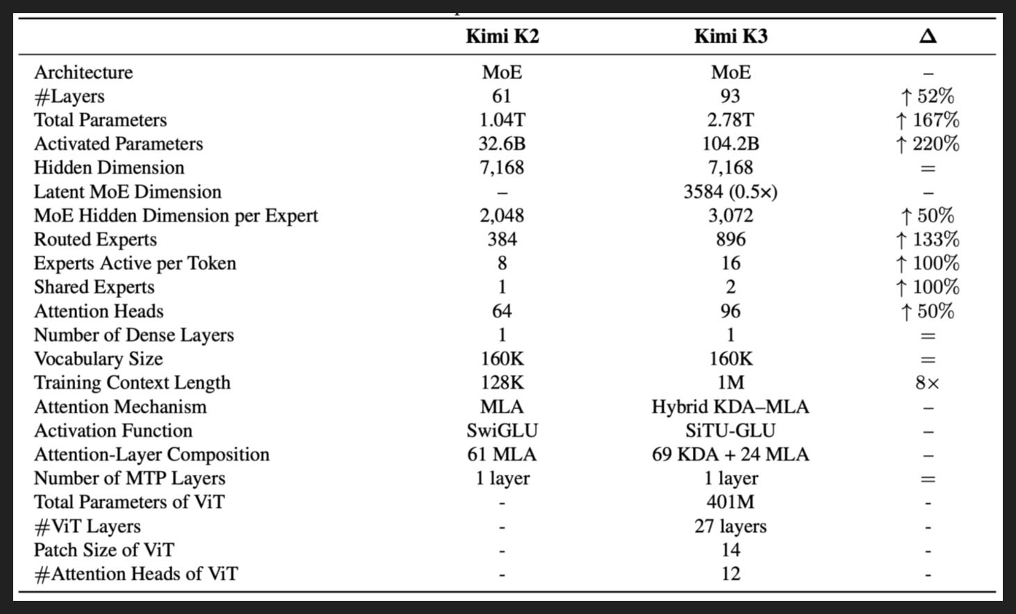
So the big story with Kimi K3 is just how big they made the model. Like look at the last column, the delta between K2 and K3. Every single numerical dimension is bigger, sometimes dramatically so.
The headline is of course that 2.8T parameters, which they achieved by making the model 52% deeper and having 133% more experts, each of which is 50% bigger. So the model is thinking more deeply about each token and has more fine-grained expertise.
The activated parameters also went up, mostly from having bigger experts and selecting more of them at a time: double the experts active per token.
On more of the catch-up side, the context window is now 1M tokens - standard by now for frontier models - and Kimi now comes with vision natively trained in rather than glommed on.
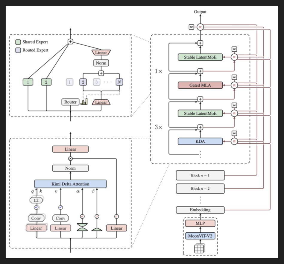
Here’s the architecture, which we should mostly be prepared for at this point.
In the bottom-left we have Kimi Delta Attention. In the top-left we have the mixture of experts, with two experts always active and the rest selected based on the input. They have a couple tweaks here which I’m going to skip over, but the tweaks are why they call theirs Stable LatentMoE instead of just MoE or similar.
Now on the right we have the entire model. It starts with the vision encoder and then the embeddings, then it has a series of transformer blocks, then the output - standard stuff. There are two things to note.
One is what’s in each transformer block. They open it up in the top half, that section with KDA and Stable LatentMoE and Gated MLA. What they’re saying here is that in each block, they do KDA + Stable LatentMoE three times, then a more standard version of attention called MLA + Stable LatentMoE one time. Because MLA has the traditional KV cache, albeit a compressed version, it captures global context in more detail. It’s pretty common nowadays to have this mixture of cheaper attention with a bit of higher-quality attention, and 3:1 is probably the most popular ratio for it.
So that’s one thing to note. The other is all those lines on the right side: the attention residuals. Kimi K3 actually uses attention residuals on a block level rather than at every individual layer, as a compromise between cost and quality - similar to using a mixture of attention types as we just saw. This 80/20 rule kind of stuff is a recurring theme in LLM architecture innovation.
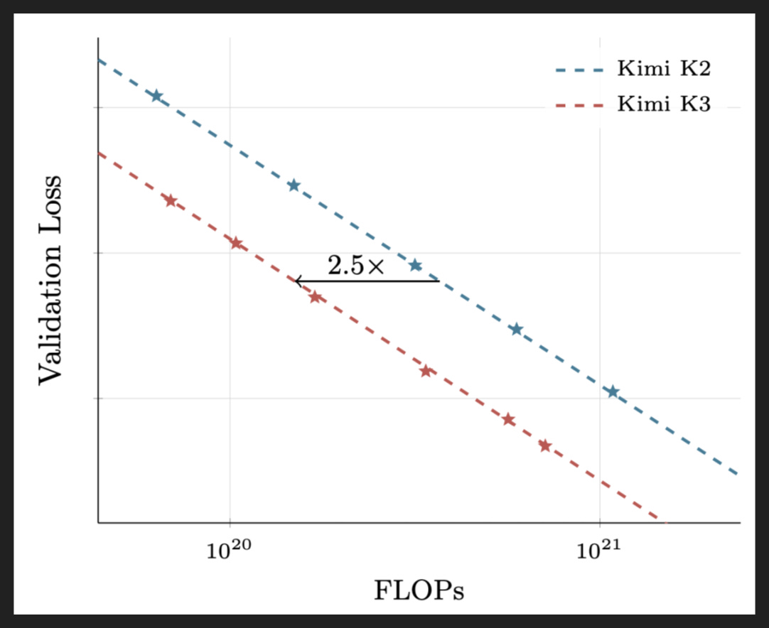
So here’s one big payoff due in part to their architecture changes: a 2.5x reduction in pretraining compute to reach the same level of performance for K3 compared to K2. Of course data and infrastructure efficiency had an impact too, although we don’t know the breakdown.
Of course what we’d like to know is how much better performance is for a given level of compute, since the compute is what we control and budget for, but without units on the y axis we can’t say. However, based on the stars on the two trendlines, it seems K3 got better performance for less compute compared to K2. So it’s a win on both dimensions.
I also just want to say how crazy it is that scaling laws are so predictable. Look how straight those lines are! I know log plots can hide a fair amount of deviation, but still.
Before we move on to post-training, you may be wondering where the detail on pretraining data went. Well, there basically isn’t any - three short paragraphs with no numbers whatsoever is all we get. The only interesting bit in there is their call-out of “programmatic multimodal data”, things like games and 3D renders and CAD that one can describe and generate with code. CAD in particular is having a moment right now for frontier models.
Now let’s move on to post-training. They follow the emerging standard for frontier models: some SFT, a ton of RL to create teacher models across different domains, then multi-teacher on-policy distillation (MOPD) to create one final model that effectively covers all domains.
The SFT section is small and sparse, again bereft of numbers. They do mention a focus on agentic tasks - no surprise - and verification with humans in the loop.
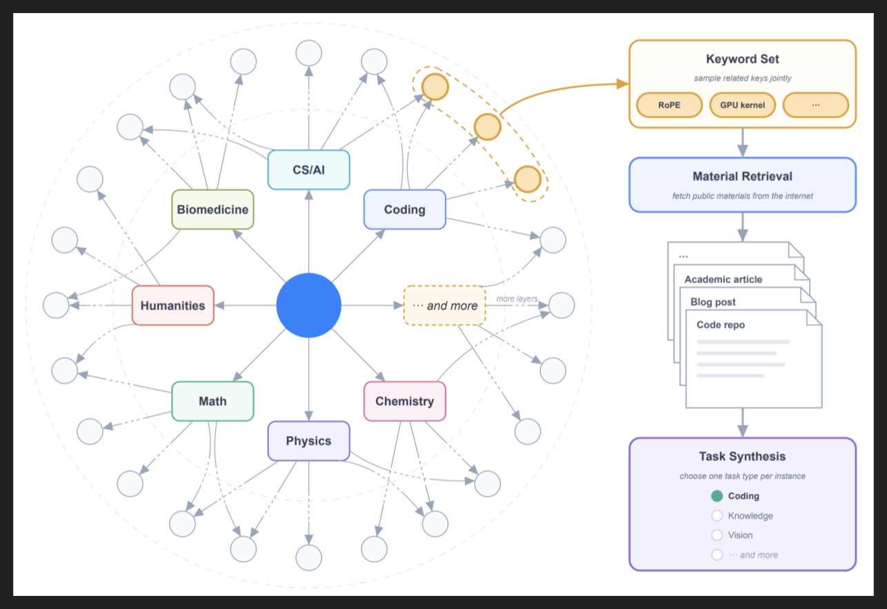
Thankfully they spend much more time on RL. The graphic here describes how they create RL tasks. They also have RL environments, which I’ll come back to.
So for the RL tasks, they start out with a knowledge graph - basically a map of increasingly granular concepts, built automatically by specialized agents that keep distinguishing concepts until they feel the concepts are atomic. Once your knowledge graph is complete, you can sample individual nodes or nearby groups of nodes to determine what your task will cover. In the example here, it’s mostly coding with a dash of AI, which produces some LLM jargon like “RoPE”.
The keywords seed a search for relevant materials. Searching the web and in-house databases yields source material, which yet other specialized agents synthesize into tasks.
No idea how much data they actually made, and nothing in here is revelatory, so they’re clearly keeping many details to themselves. That’s the difference between open weights and open source!
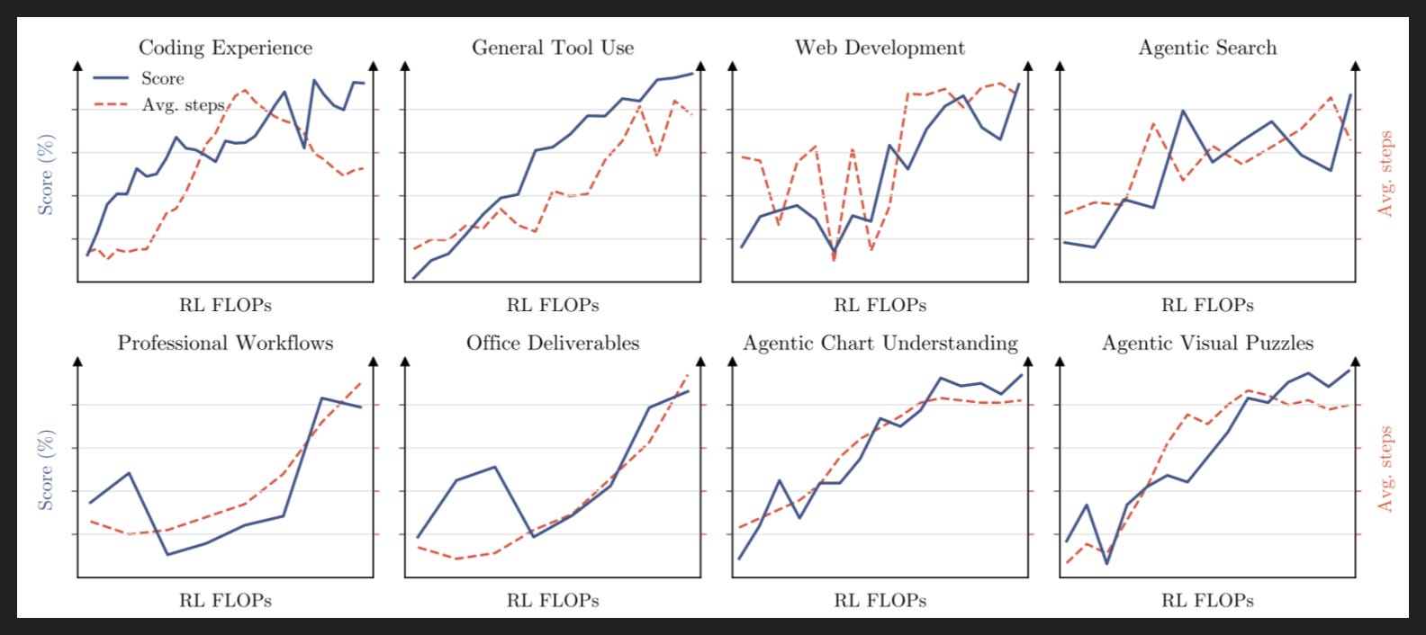
So their RL focuses on three broad domains: general tasks, general agents, and coding agents. “General tasks” includes basic stuff like instruction following and vision and tool use that we now take for granted in model capabilities. It’s only with the latter two domains that we see real work like web development and deep research.
As you might expect, they have the teachers for MOPD split across domains. The other way they split up teachers though, which I’ve not seen before, is by reasoning level: low, high, and max. So three domains times three reasoning levels equals nine total teachers.
It is these nine teachers that get the RL shown here. The RL happens in a few different environments, each with the appropriate tools and data. For example, Web Development has web dev packages and a way to render what the agent produces. It also has deterministic checks where applicable and model judgment otherwise, like for evaluating the visual design of a web game. They do mention the judge uses a rubric, but the judge is the one creating the rubric in the first place - no evidence of human data here.
They do give a bit of color on some environments. For example, the personal assistant one has mock implementations of Gmail, Slack, Notion and the like. They have another one designed for agents to progressively submit, see results, and improve upon some work, like speeding up certain GPU operations. I have a graph about that on the next slide because I think it’s a wider trend.
One other interesting bit about their RL environments is they include several different harnesses: not just their own harness, Kimi Code, but also Claude Code, Codex, OpenClaw, and Hermes. So they built Kimi K3 to work in many setups. We don’t know for a fact, but it’s unlikely OpenAI and Anthropic are putting in the same effort to make their models portable across harnesses; my guess is they do the opposite and train their model to expect their harness.
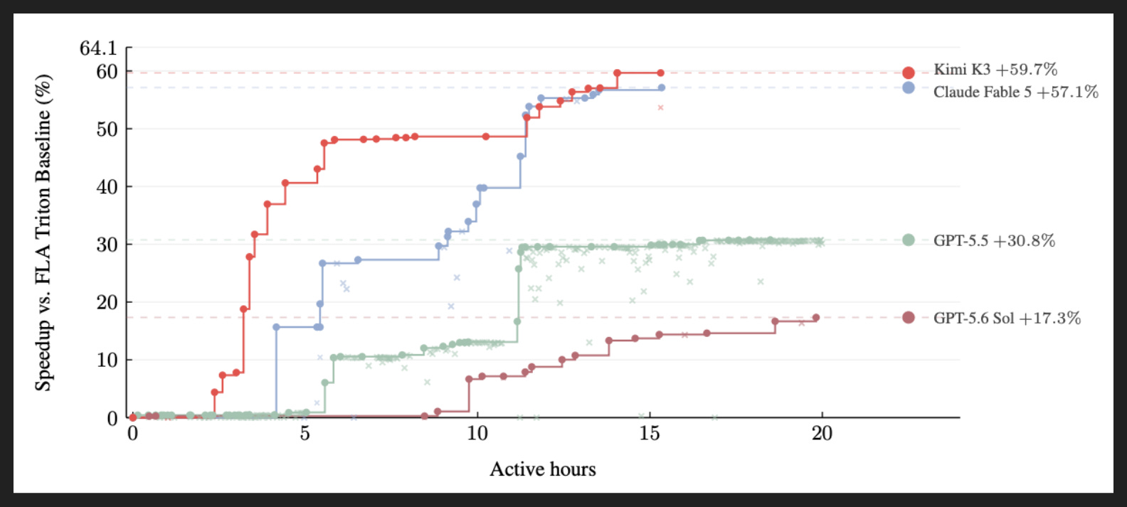
Here’s that graph I promised about iterative improvement on GPU operations. On the x axis we measure how long the agent has been operating, although number of submissions or number of tokens would also work - anything to indicate duration.
On the y axis we have the relative percent speedup for the GPU operation. Each dot is a submission, and the line connecting many of the dots is the frontier, i.e. the maximum speedup so far. The difference is particularly clear for the blue and green trends, where many submissions fall below the frontier.
This type of task and graph is increasingly common, popularized by Andrej Karpathy’s Autoresearch harness. I expect to see a lot more graphs like this, especially as more work goes into recursive self-improvement (RSI) - which is exactly what Karpathy joined Anthropic to work on.
Relatedly, the authors note in the paper that Kimi K3 actually was optimizing its own performance during development, so these results aren’t in a vacuum - they are live in production and pointing to the RSI dream.
I also think more generally we will see more focus on a few hard examples and how they demonstrate model capabilities in the way benchmarks do now. As each task becomes more difficult and longer, there will be more to analyze on each one and it may be impractical to generate a benchmark’s worth of tasks. In the extreme, you have problems with specific names like the Riemann hypothesis or Navier-Stokes.
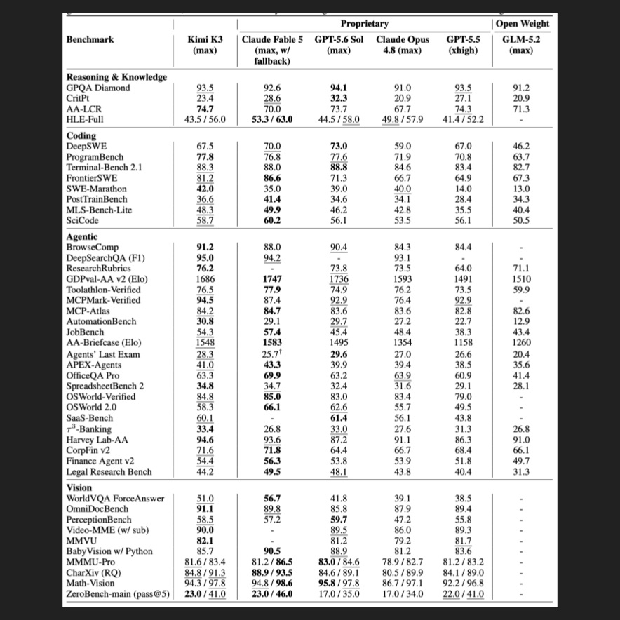
For now though, benchmarks are still plenty useful, so let’s quickly look at them. We already know the aggregate story from the background slides on ECI and Artificial Analysis, but I always like to look at which benchmarks are “in circulation” so to speak.
General agentic ones, which they just call “Agentic”, take up the most room and reflect the variety of tasks people are using agents for: research, spreadsheets, computer use, customer service, law, finance, and a smattering of other white collar work. (I have covered Agents’ Last Exam and OSWorld 2.0 previously.)
Agentic coding, which they just call “Coding”, gets its own section and includes benchmarks on ML and scientific programming. Again, indicative of where agents are going and where labs want to focus.
I’ll also call out the Scale benchmarks I see, namely Humanity’s Last Exam and MCP Atlas.
One thing I expected to see more of was some coverage of multi-agent swarms. They mention two relevant internal benchmarks elsewhere, and one case study has a single line about using subagents, but given their past emphasis I was expecting a much deeper dive. Funnily enough, Kimi K3 came out the same day Hugging Face disclosed a massive hack by a swarm of AI agents, now known as the Hugging Face incident. Probably just a coincidence that Moonshot chose to report less on swarm performance here than in previous tech reports though.
Perhaps relatedly, the paper does mention Kimi K3 discovered 16 previously unknown vulnerabilities in important software packages, including a subsystem within Linux. Finding vulnerabilities seems to be a natural benchmark these days.
That’s it for what I want to cover, but the paper has a ton more detail on their infrastructure, which they stretched to the limit with the massive number of parameters, the many extra experts, and the octupled context window. If you want a taste of why ML engineers make such bank (and why ML companies want to automate them), just take a look at section 5.
My Takeaways
Kimi K3 has raised the bar for open weights model size, which others are sure to follow
Qwen3.8-Max is already 2.4T
I expect DeepSeek at minimum to release something in the 2T range (current max is 1.6T)
GPU and RAM prices are not coming down any time soon
Kimi models will likely continue to be the top choice for companies that want to post-train their own near-SOTA models
Autoresearch-like graphs are here to stay
Already seeing work like this in the wild
I’m expecting to hear more about single tasks in the same way we currently hear about benchmarks