

EdgeBench: Unveiling Scaling Laws of Learning from Real-World Environments
or, Learning to Learn From Experience

Originally presented as a live talk on July 22, 2026

Background
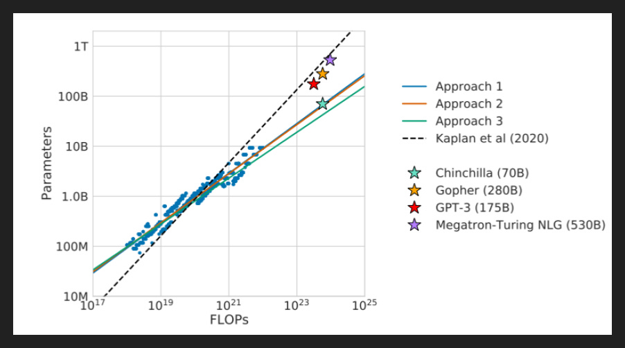
I want to start with the notion of scaling laws and how they relate to technology itself.
In the narrow sense for LLMs, scaling laws tell us how to optimally balance compute, data, and parameters as we scale up our efforts. Like whatever your constraint is - typically it’s the compute budget you have for pretraining - your other optimal settings fall out of that. So if we have a certain number of FLOPs, which is the standard unit of compute, then using the scaling laws we can calculate the model size and the number of tokens that will minimize the loss.
That’s incredibly useful for anyone trying to build an LLM. If scaling laws didn’t exist, and you had to find the right balance empirically, you might spend months just trying different combinations every time you wanted to pretrain a new model.
The scaling laws are also pretty much independent of model architecture, at least within the transformer family. The laws are not 100% exact, so it’s more like the error bars cover all the changes people are always making to different parts of the architecture and training recipe and so on, but broadly speaking they’re quite robust.
The graphic here is from the most famous scaling law paper, Training Compute-Optimal Large Language Models, better known by the name of the model they trained in the paper: Chinchilla. In the paper, they improve on a previous result by Kaplan et al, and they show that recent models are undertrained, meaning they are too big for the amount of training compute they received. The Chinchilla model, despite being less than half as big as GPT-3, significantly outperforms it.
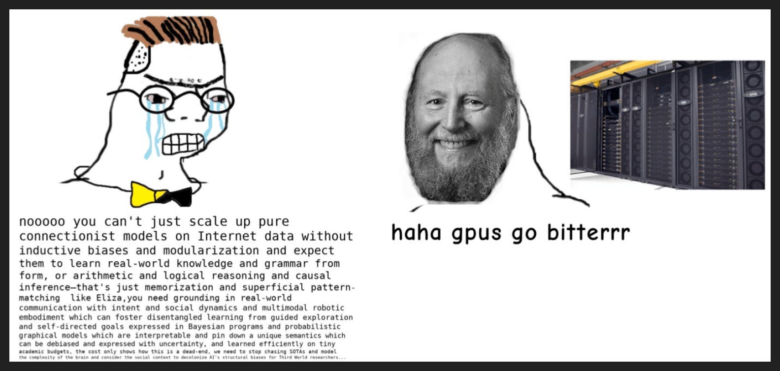
There are many other specific scaling laws - we’ll cover one in the paper today - but more broadly is the lesson of scaling in general.
Its most famous avatar is The Bitter Lesson, a remarkably brief essay from 2019 by pioneering AI researcher Richard Sutton. It opens with the following lines:
“The biggest lesson that can be read from 70 years of AI research is that general methods that leverage computation are ultimately the most effective, and by a large margin. The ultimate reason for this is Moore's law, or rather its generalization of continued exponentially falling cost per unit of computation. Most AI research has been conducted as if the computation available to the agent were constant (in which case leveraging human knowledge would be one of the only ways to improve performance) but, over a slightly longer time than a typical research project, massively more computation inevitably becomes available. Seeking an improvement that makes a difference in the shorter term, researchers seek to leverage their human knowledge of the domain, but the only thing that matters in the long run is the leveraging of computation.”
Did you catch that? He’s saying scaling of compute is the baseline assumption, and any work we do better take that assumption into account, or else it will only matter in the short-term until scaling catches up.
Sutton gives a few examples. In chess, “brute force” search-based methods dominated methods that encoded centuries of human chess wisdom. In Go, a similar story occurred. In speech recognition, learning eventually beat the methods based on human knowledge. In computer vision, much the same happened.
In all cases, work that took advantage of the inevitable increase in compute outlasted work that made efficient and scrupulous use of the compute of the day, acting as though the “inefficient” and “brute force” methods would never become feasible.
In my view, this is the major trick in the tech playbook: work a problem until the only constraint becomes resources, then dump resources into the problem. A machine where the bottleneck moves around a lot isn’t much of a machine at all; it can’t deliver predictable results and thus requires a human at the helm. A true machine does its work reliably and can do more work the more fuel you give it. We are all living through a period of scaling right now with the way everyone is building out data centers.
Scaling may not continue forever, but at least within some regime, we want scaling and we want to know the scaling laws, to design bigger systems and to forecast future performance.
It’s always a bit funny how some scaling laws work. Like with the Chinchilla scaling laws, that seems to be a natural property of the universe, more akin to a physical law. But for Moore’s Law, which underpins The Bitter Lesson, that’s a prediction about society and how it will continue allocating resources, in scientific discovery and also in hardware production.
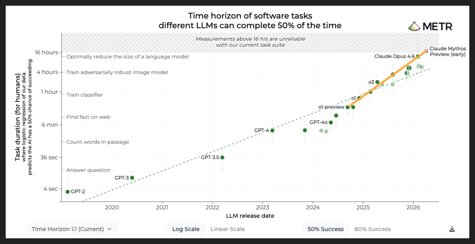
The famous METR graph is a scaling law of the latter type. As I’ve covered before, this graph shows how models are becoming more and more autonomous over time, able to handle increasingly long-horizon tasks as measured by how long it takes a competent human to do them.
The current results are actually somewhat in doubt - Mythos is too advanced for METR’s measurement task suite - but we do have reliable data points all the way up to Claude Opus 4.6, which came out in February 2026.
Now the METR folks show just the one fit line, one scaling law. But arguably there is a break in the line, which I’ve drawn in orange, with growth at 10x/year, meaning by February 2027 we’ll have an agent that can do about 100 human-equivalent hours of work autonomously at 50% success rate. Pretty nuts.
Anyway, that new trendline starts with the introduction of reasoning models. See, o1-preview introduced another axis of scaling: not training compute, not data, not parameters, but inference compute - how long the chain of thought could get and still improve the final answer.
That’s the other part of the scaling law puzzle: where is everything we could scale? Because once we find them, we can dump more resources into them and juice performance.
Now in the course of these increasingly long tasks agents can do, there is plenty of trial and error. In some ways that’s what makes agents work: interacting with an environment, gaining information, incorporating it into future actions. That sort of exploration and iteration isn’t really present in chatbots, and it’s also not part of classic benchmarks where you’re supposed to respond to a prompt in one go.
Of course models have always been able to adapt based on their context; even responding to a basic prompt is in a sense adapting behavior to context. Historically the most common tactic has been to write rules and provide examples to put in the prompt, which folks call “in-context learning” and sometimes “few-shot” or “many-shot” depending on how many examples are in the prompt.
But now there’s this dynamic element, where an agent’s experience within the same task becomes part of learning. Maybe the learning goes in a scratchpad just for the task, maybe it goes into a long-term memory system, maybe it just stays in the trajectory and survives compactions. However it happens, the agent is learning as it works, just like a human would.
Sometimes people call this continual learning, although sometimes I see that term specifically for learning into the weights, i.e. training the model. That’s not what we’re talking about here. What we’re talking about is all ultimately in the context window, although it may live in a different tool and only enter the context window when the agent calls the relevant tool to fetch it.
Continual learning is crucial because lots of important context will never make it into the training data. Like most businesses are not going to fine-tune a model on their business logic and proprietary information. So that information has to come through the context window.
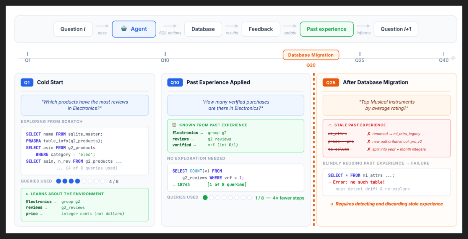
The graphic here is from Continual Learning Bench, a bit of prior art in this space, which measures an agent’s ability to learn information from one task in a domain or environment and apply that knowledge on another task. So in this example, for the first query, the agent learns some stuff about the database, shown in the green box. Then for the second query shown, with label Q10, that green box of knowledge appears at the start to inform the agent on the task. Later on, with label Q25, the agent has to recognize which information is now stale.
For CL Bench, they test different models but also different context management systems, including Claude Code and Codex, which are coding agent harnesses but include many tools and techniques for managing context, like memory. They find that pure in-context learning, i.e. just keeping everything from the trajectory in the context window for as long as possible, does the best. However, there are only six different tasks, although each one contains many different “instances” - like Q1 and Q10 and Q25 in the diagram. And each instance is not that long, so even though an overall task can be quite long, the continual learning is more like a shared base for each instance rather than one long narrative.
So models apparently have this continual learning ability. But as we know, with agents, the model is only half the story; the other half is the harness.
Many agent harnesses improve continual learning, but usually as a means to improving performance on the agent’s focus area, like coding as with Claude Code. But there is one famous harness whose main job is arguably to improve continual learning: Autoresearch, from Andrej Karpathy.
The idea of Autoresearch is quite simple: plan an experiment, run it, observe the results, and use the results to plan a new experiment. It’s the scientific method, but encoded into a harness. The human picks the goal and hands off the rest to the agent.
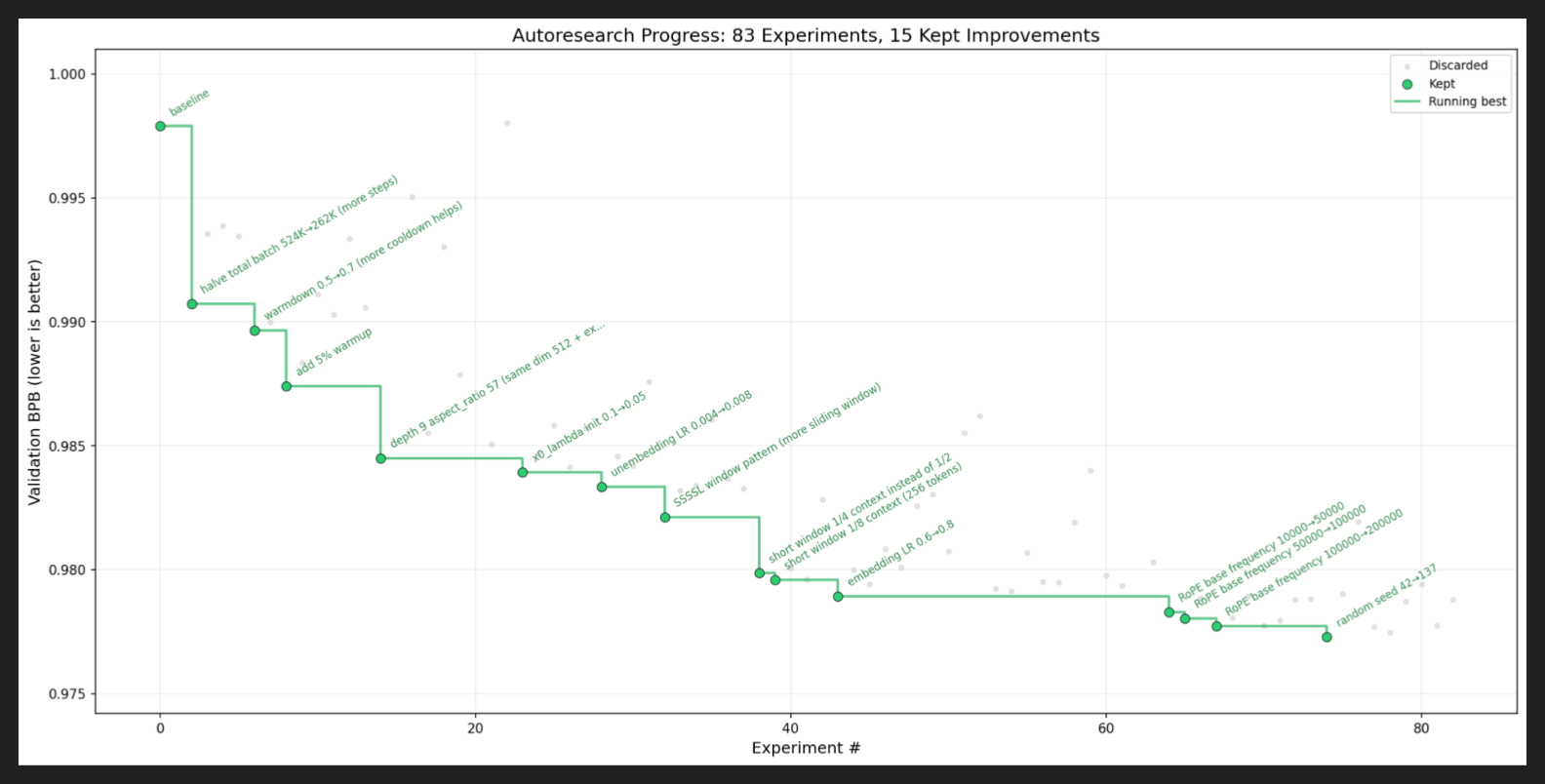
In the actual Autoresearch repo, the goal is to train a version of GPT-2. But the general method applies to any problem with a clear metric to optimize. In the graph here, that metric is the loss, which is the classic metric to minimize when training any LLM. We will see a version of this graph later, but flipped, since the goal will be to maximize a score rather than minimize a loss.
The Paper
Since this is a benchmark, let’s start with the tasks.
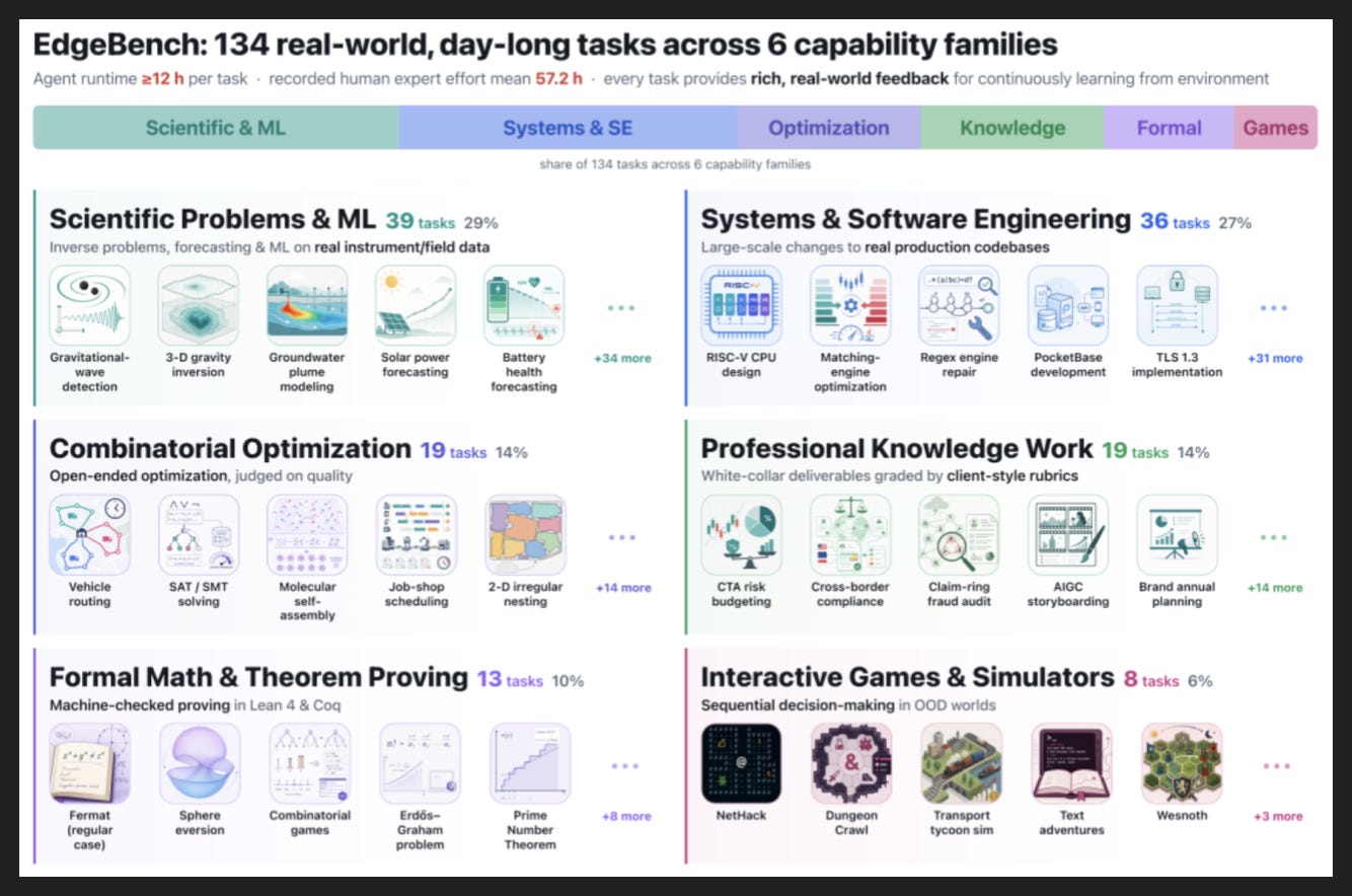
We have 134 of them, sourced from experts in many fields, with mean human effort clocking in at over 57 hours. So these are substantial tasks, putting them at the leading edge of the benchmark task time horizon distribution. We recently covered Agents’ Last Exam, and they were bragging about how a few of their tasks made it to the weeks timescale.
As we’ll see, it’s important for EdgeBench that an agent not solve any task on the first try, because what they’re measuring is ability to learn from feedback. So duration is more than just a way to match difficulty with agent capabilities - it’s intrinsic to the purpose of the benchmark.
Now as for domains: unsurprisingly, given the likely personal networks of the researchers, the tasks skew STEM, with science, programming, and ML representing over half the tasks.
Many of them are multimodal, but the authors specifically note that “tasks whose primary difficulty lies in visual understanding, especially GUI operation, are excluded” - they want the hard part to be reasoning and iteration rather than pure discernment. To me that presents somewhat of a challenge with their Interactive Games & Simulators bucket, but they don’t explain any further.
Sadly for us, there is also little detail about how they made the benchmark.
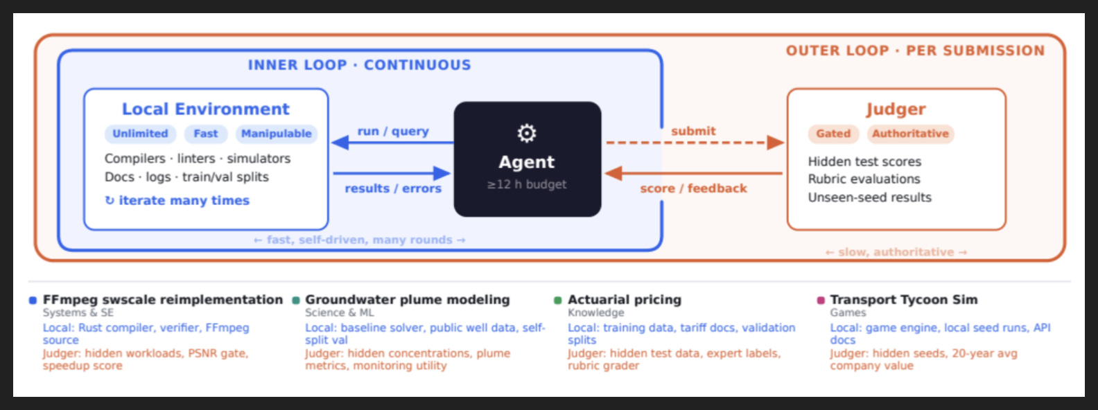
Through manual effort, the tasks become environments, where the agents are free to experiment. The diagram shows an inner loop on the left in blue, where quick feedback from tools helps the agent learn the environment better. You can see examples in blue text along the bottom.
At a slower cadence, there is an outer loop, shown on the right in orange, where the agent can choose to submit its work to a judge. The judge evaluates the agent’s work against the ground truth or rubrics or similar, then returns the score and feedback. The ultimate goal is to maximize that score. The agent can submit any number of times, although there is a cooldown period of two minutes between submissions. Again, there are examples along the bottom in the relevant color.
So both loops allow for continual learning. Of course, since this is a benchmark, we have right answers in the outer loop to compare to. In the real world, where the right answer may be unknown, you can at least shoot to maximize some metric like we saw with Autoresearch. You just have to be careful of Goodhart’s Law and mistaking the optimized metric for the thing you actually want, if the two aren’t identical.
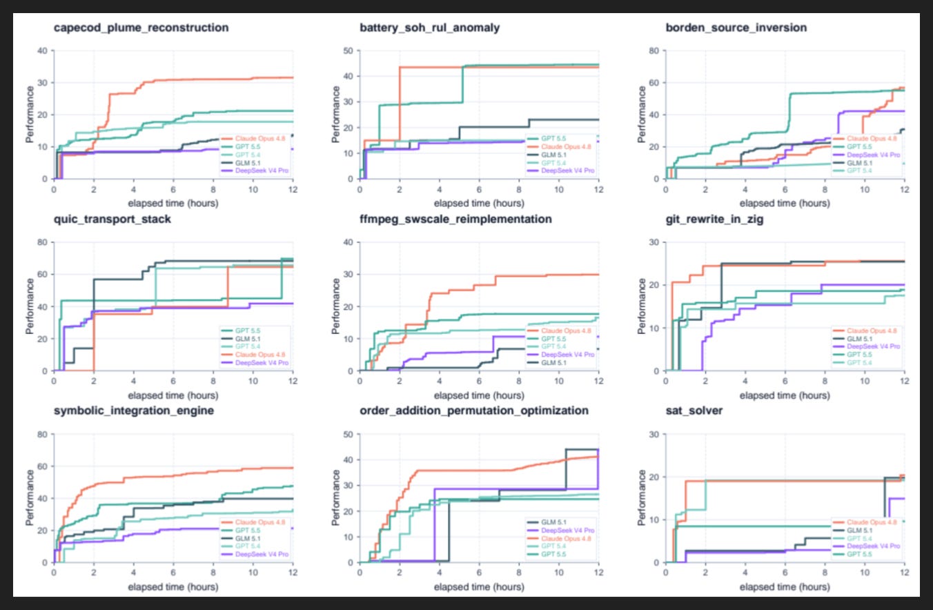
Here are the Autoresearch-esque curves, showing how top performance per model rises over time. Note how chunky the graphs often are; progress seems to happen in punctuated equilibria rather than in smooth steps, at least at a per-task level.
The keys only show the model, but the harness and context window are important too. So in full, we have:
GPT + Codex @ 256k compact window
GLM-5.1 + CC @ 200k compact window
DSv4 Pro + CC @ 200k compact window
Opus 4.8 + CC @ 1M compact window
They show later on that 1M provides about five percentage points of advantage over 200k, with a slow and steady decline in that gap as time elapses.
I’m a little surprised they didn’t use a neutral third-party harness here, but I do think there’s value in shooting for maximum performance rather than controlling variables. Just more evidence the model and the harness are becoming one integral whole.
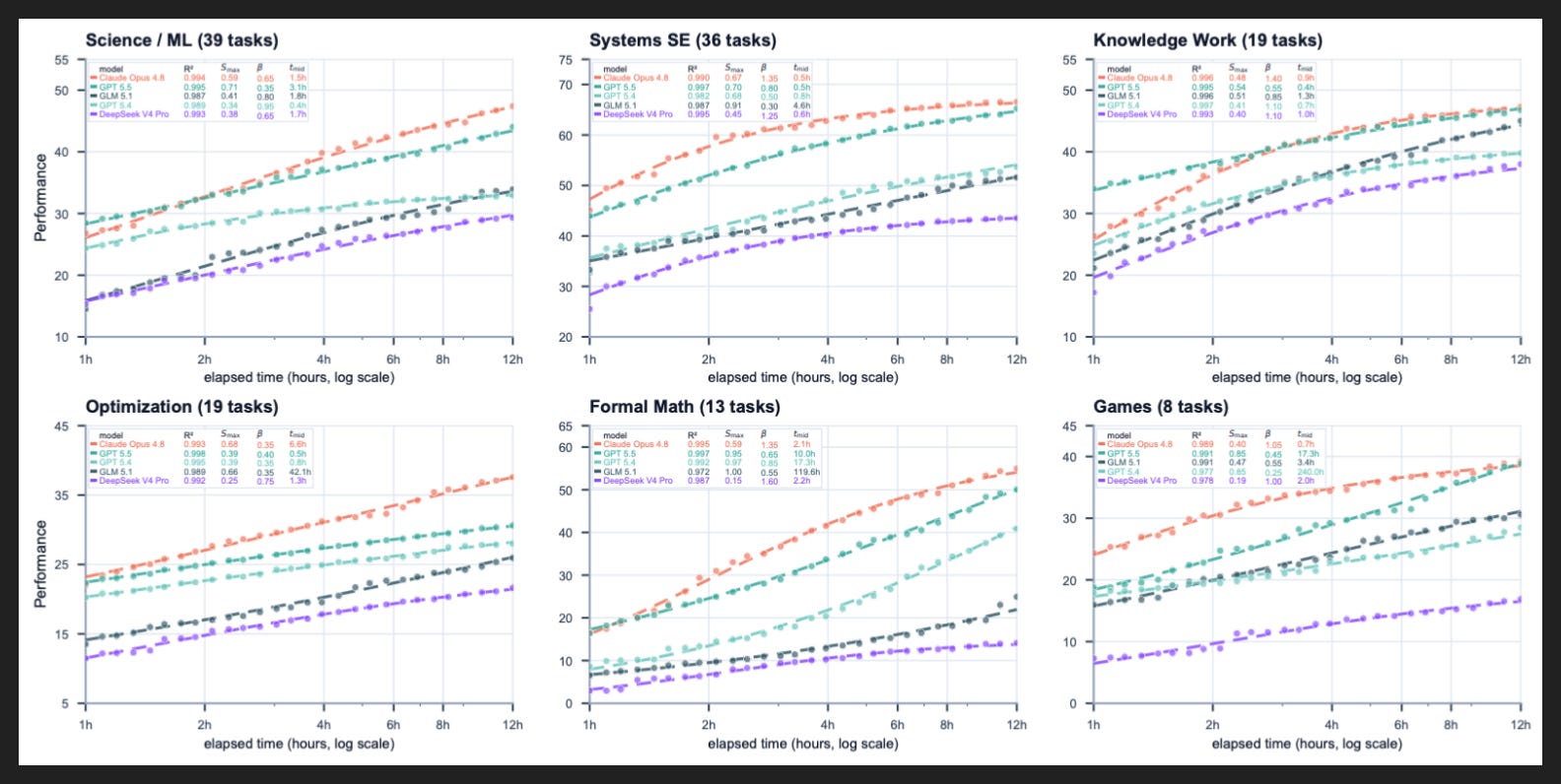
Now if we zoom out a level, from individual tasks to task categories, we see much smoother curves. In fact, they’re so smooth that you can tightly fit the same type of curve to all of them: the log-sigmoid.
A sigmoid is a classic S-curve, starting at zero and then accelerating to a midway point, then decelerating and leveling out. A log-sigmoid is that but on a logarithmic x axis, like in these graphs. So basically these models all form S-curves in log time.
That’s remarkable, because the individual tasks graphs didn’t seem to show much of a pattern at all. But if you aggregate just enough, the common pattern emerges. They have some results later showing that the pattern isn’t guaranteed from the aggregation, that it’s a real trend in how agents learn over time and over many iterations.
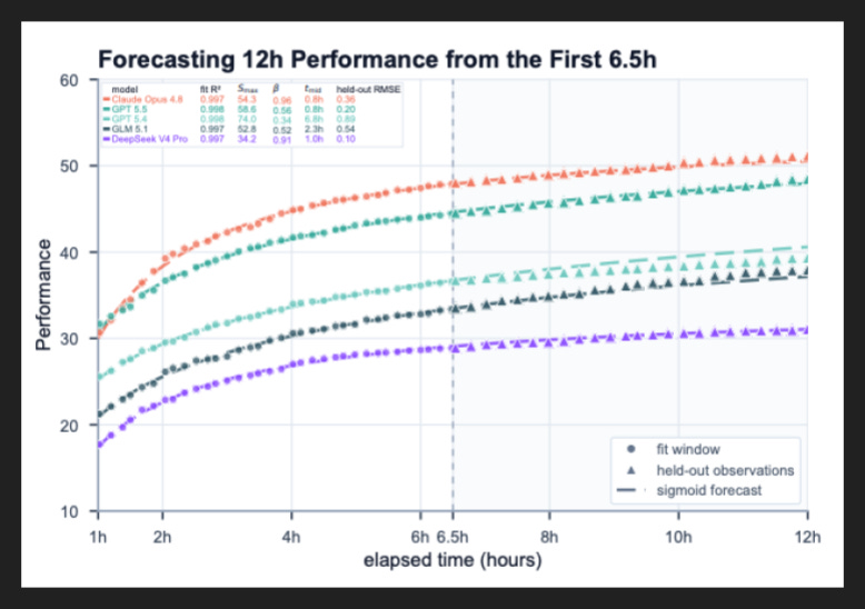
It’s also helpful, because it allows us to predict performance past the 12-hour window, which really saves a lot of time and tokens compared to having to actually hit 18 or 24 or 72 hours.
Here’s a validation of the predictive power of the fitted curves, taking performance through a 6.5 hour window and projecting it forward to 12 hours. The curves are pretty dead-on, even for the most inaccurate one, GPT-5.4 in teal. And actually they explain that for GPT-5.4, the score was lower than expected due to API flakiness rather than poor model performance.
So not only do they empirically validate their scaling curves, they also provide a theoretical justification. I don’t want to spend too much time on it, but the broad idea is to represent different bits of knowledge and insight as nodes on a graph. Any prerequisite knowledge is a connection. If you assume the graph structure is self-similar, basically that it looks roughly similar throughout, then you naturally expect a log-sigmoid shape when you chart progress through the nodes over time.
They’re not rigorously proving that every task will follow these laws, in part because some graphs will not be self-similar, but self-similar graphs are common enough that the theory explains why log-sigmoids are plausible at sufficiently high abstraction.
So we have scaling for a given model over the elapsed task time. That’s nice for understanding a model’s performance ceiling, and it saves us some experiment time, but there is a juicier finding in EdgeBench.
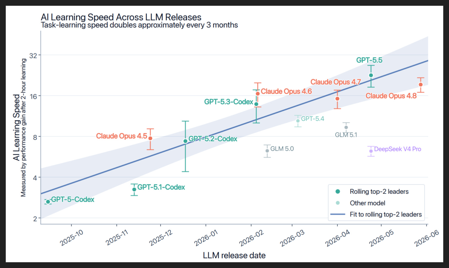
Specifically, it’s this chart, basically their version of the famous METR graph we covered in the background portion. What this graph shows is how quickly a given model learns, as measured by average performance gain on a select subset of tasks within a two-hour budget per task.
What they find is that newer models are consistently pushing the frontier, doubling the learning speed about every three months. That’s 16x/year, which is faster than the METR graph at 10x/year. So if the trend holds, not only can we expect agents to accomplish longer tasks as measured in human completion time, we can also expect agents to complete the same tasks more and more quickly - and that’s before taking parallelism and multi-agent systems into account!
Now one thing to keep in mind is they aren’t measuring pure model performance, or even model + harness performance; they are also measuring hardware performance. Like if two equally capable agents are competing, but one gets twice the token output speed, it will finish significantly earlier.
In practice though, OpenAI and Anthropic shoot for similar output speeds unless you pay extra for faster tokens, so I think these results hold. In fact, the only result I would caveat is for GPT-5.4, which as we discussed encountered API issues and thus has a lower score than expected. So if you imagine the datapoint for GPT-5.4 on this graph a bit higher in the world where the API didn’t flake, it fits the trend quite well.
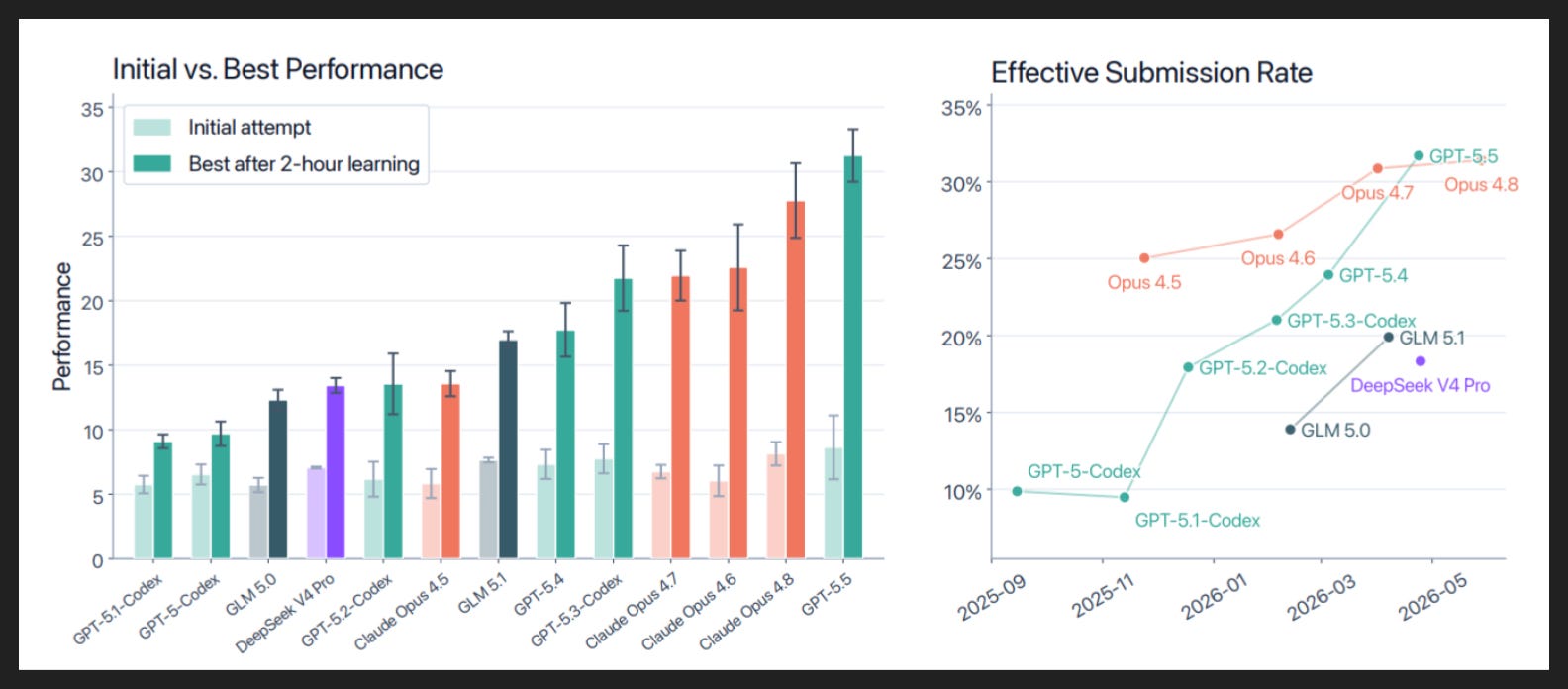
On the left is another look at the same data, showing performance at the start and end of the two-hour window. The researchers selected the subset of tasks based on how similarly all the models initially did, so if new releases start to do significantly better to start, they may have to swap out the subset. But for now the initial performance seems about even, and there’s plenty of performance ceiling to go.
On the right though is a new trend, showing how effective new submissions are. Specifically, the graph shows what percent of submissions in the outer loop improve performance. So it seems newer models are more likely to make submissions that improve their score. Here is how the researchers put it:
“Stronger agents use feedback more deliberately: they build a submit-ready baseline, preserve the current best solution, make focused changes, and use feedback to keep gains or roll back failures. Weaker agents more often over-trust local proxies, bundle unrelated edits, or continue broad exploration after feedback has ruled out a direction.”
I do think it’s a bit confounded whether newer models just have better work and thus better submissions vs having better discretion on which work to submit, but either way you as a user are more likely to be looking at better work.
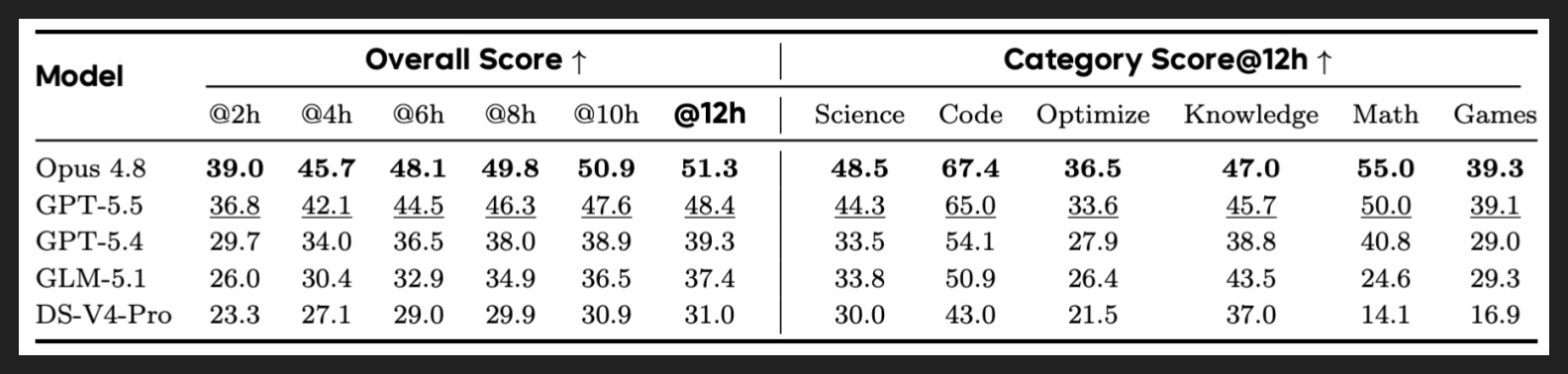
We do have a leaderboard of course, given this is a benchmark, but honestly it’s not really the main story here; the big finding is the scaling laws rather than any one point in time.
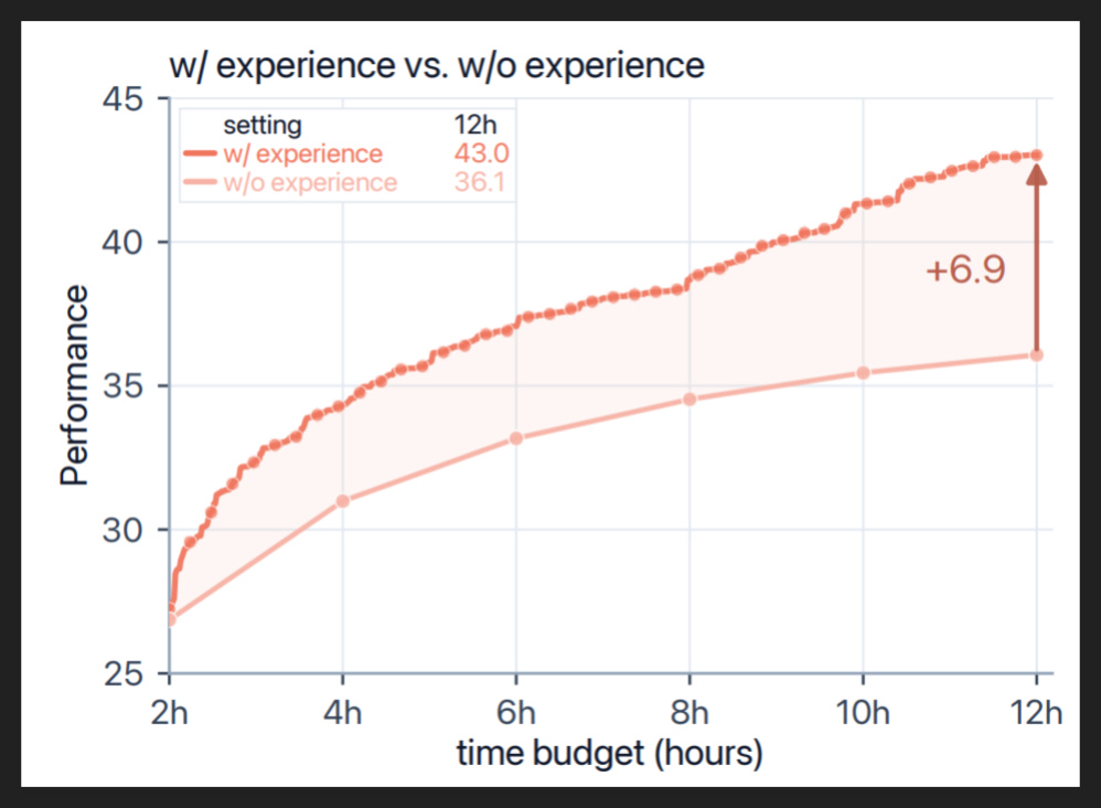
Now of course with more submissions you’re likely to improve your high score. So the question for continual learning is, how much does it help to see your previous work and submissions? What is the impact compared to the baseline of many independent attempts, where you only get one outer loop submission?
Here they answer that question, using Opus 4.8 to test. The lower curve, comprising independent submissions, is basically pass@k but with k as a function of time. And it displays the classic diminishing returns curve of most pass@k results.
Meanwhile, the upper curve comprises dependent submissions, i.e. where the agent sees the results of each outer loop submission and can continually learn. Here we see a consistent and perhaps even widening gap, where more experience pays dividends. So yes, purely providing more chances does improve performance, but not as much as continual learning does.
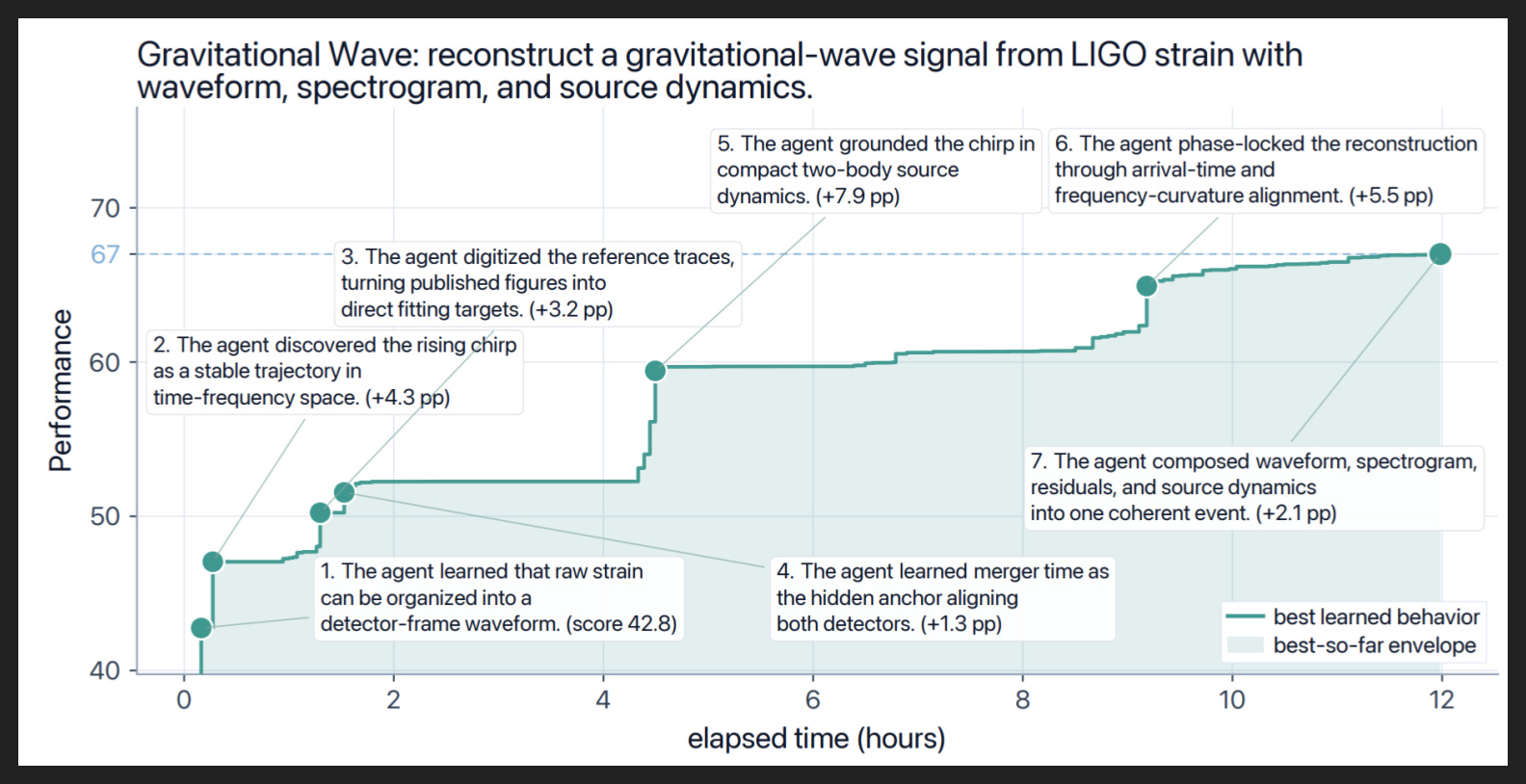
Finally, let’s zoom in on one task example, with an attempt by GPT-5.5.
Here we see the classic punctuated equilibrium pattern, long periods of little or no progress with occasional big jumps, until time runs out or until the agent reaches its limits. Personally I don’t know anything about detecting gravitational waves, so the specific jumps don’t mean much to me, and I don’t think they’re crucial to comprehend.
What’s interesting about this example task though is the high-level strategy GPT took to partially solve it. The authors list four points:
The agent first makes the problem measurable before making it better
When direct repair stalls, the agent decomposes the failure into searchable subproblems
Identifying a main bottleneck lets the agent keep searching productively
After finding a stable solution, the agent keeps the core and repairs only the remaining errors
To my eye that’s quite a general and broadly applicable set of steps. I wish they had distilled more examples like this, or perhaps taken these points and checked how pervasive they were in other attempts, by GPT and by other model families. I also wonder if prompting the agent to use these techniques would improve things.
My Takeaways
We may have a new METR to track
Why is METR having trouble with sufficiently difficult tasks, but EdgeBench was able to produce them?
Unclear what specifically makes learning rate scale
Model (training data)
Harness
Context length (they did prove this one actually)
Maybe we can add signals to increase learning rate further
More and better feedback from tools
Another agent to work with
In-context learning and error correction are mandatory
Even a 99% accurate agent has a 50% chance of failing after just 69 steps