

DSpark: Confidence-Scheduled Speculative Decoding with Semi-Autoregressive Generation
or, Diffusion in Production

Originally presented as a live talk on July 15, 2026

Paper · Repo · Hugging Face
Background
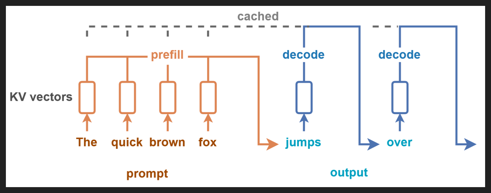
To understand this paper, we have to understand how a model on a GPU turns your prompt into predicted tokens.
Let’s start with what we already know from our daily use of LLMs: you pass in your prompt all at once, you wait a bit, and then you start getting back tokens one by one.
Already we can start to relate to this diagram. The part where you pass in your prompt is called prefill. During prefill, you are filling up the working memory of the model, what we call the KV cache. The diagram here kinda breaks up “KV” and “cache”, but you can see that the prompt turns into KV vectors, and then those get cached, hence “KV cache”.
So now we have all the input in our working memory. That can take a long time depending on the hardware you’re using and how big your input is, but importantly, prefill happens for all input tokens in parallel. Typical prefill speeds are in the hundreds or thousands of tokens per second.
So once prefill is done, the model is ready to start making predictions. And it makes those predictions one at a time, as the diagram shows: first “jumps”, then “over”, etc etc. This stage is called decode, because we’re decoding the mathematical representations that the model works with into words that humans work with.
Because decode runs one token at a time, it is much slower than prefill, typically in the tens of tokens per second.
Note that when we decode a token, it gets cached too - that’s why the dotted line at the top spans prefill and decode. So the KV cache, that working memory, grows every time the model outputs a new token.
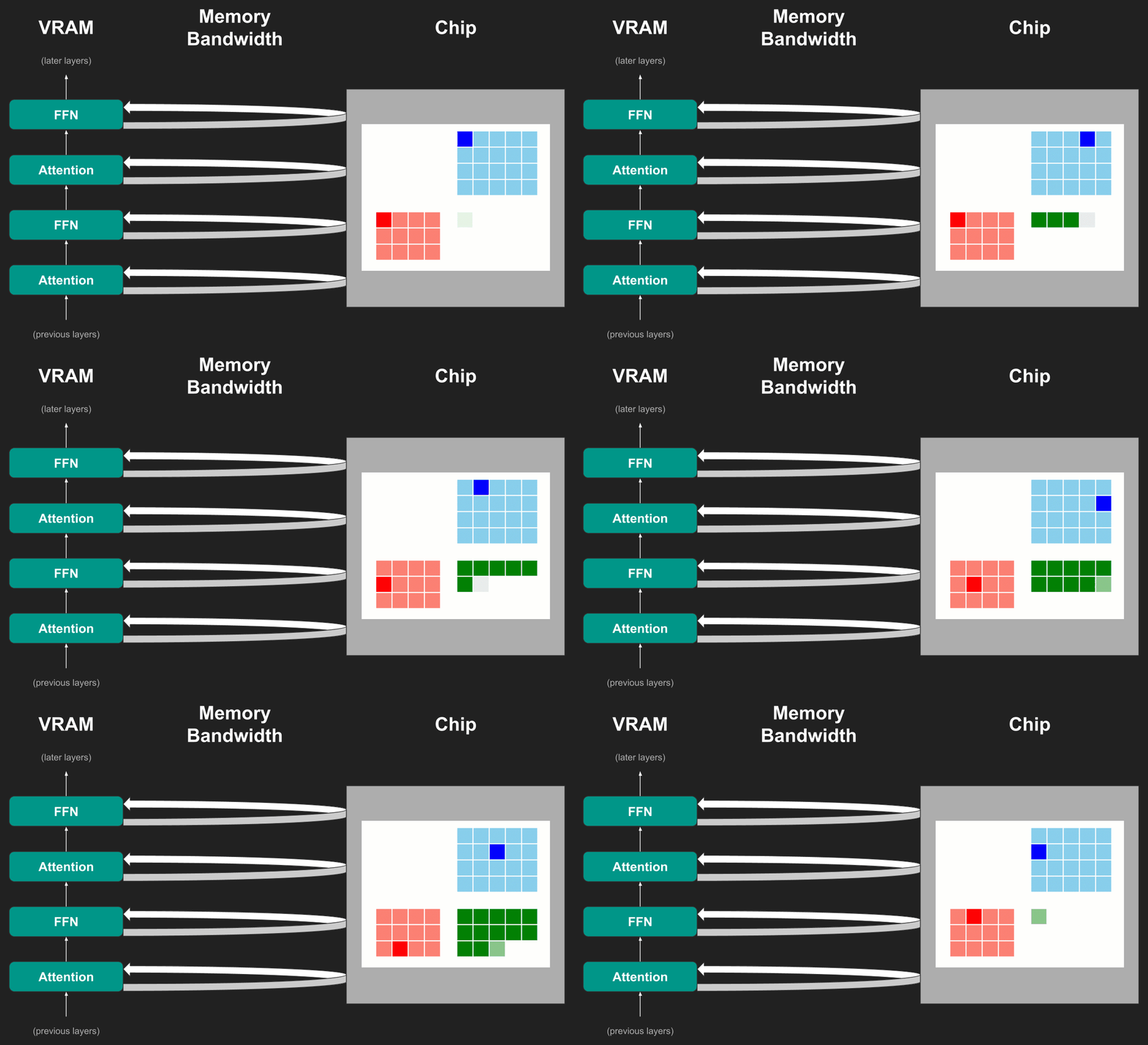
Now let’s look a level deeper, at the hardware. On a GPU, you have your chip, and you have your memory, aka your VRAM. When you start up your model server, the server reads the model from your hard drive and puts it into your VRAM, right next to your chip.
When you actually use your model, like by sending it a prompt and getting back a response, your model server takes one layer of your model at a time from VRAM and sends it to your chip for computation. So if I’m at the very first attention layer, it’s gonna take my input and the matrices that actually make up the first attention layer and send ‘em to the chip for multiplication and so on. Then it takes that first attention layer back from the chip, along with the KV cache created from the computation, and it’s gonna send in the first feed-forward layer for computation.
That process of loading and computing and unloading happens over and over again until you’re at the final layer, where the chip can finally produce the predicted token. Then you gotta do the whole routine over again to predict the next token.
So this shuttling of weights to and from the chip is typically what slows you down - the constraint is your memory bandwidth, not the speed of your chip. If you can somehow compute multiple tokens at once in decode, like you do for prefill, then ultimately you can predict tokens faster.
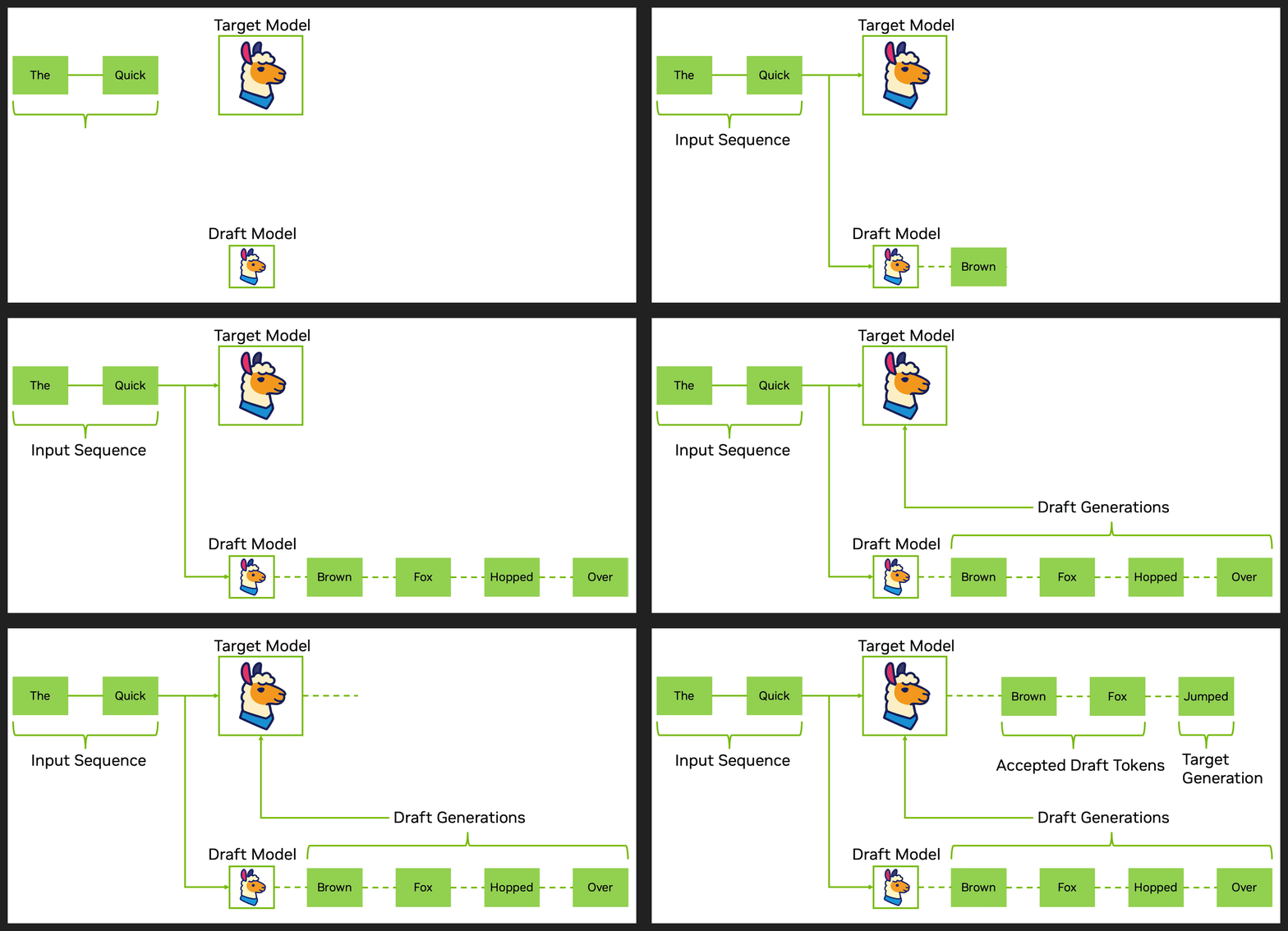
The question is, how do you predict multiple tokens? If predicting a token requires understanding all the tokens before it, how can you predict more than one?
The answer is in the name of the technique: “speculative decoding”. Instead of making a brand new prediction every time, you speculate about what the next few tokens will be - you take a guess beforehand and then check.
Speculative decoding works for the same reason prefill is faster than decode: inputs get processed in parallel. As we said before, once you load the weights onto the chip, it’s quick to do one or two or three or four calculations. As long as you have a good way to guess tokens, the model can check them all in parallel.
Of course, if the first token fails, then the other ones you guessed after it will likely be wrong and you’ll have to throw them away. But if your method for guessing tokens is cheap enough, and you’re not wrong too often, it can work out.
One common method is to have a version of the model itself make the guesses. Specifically, a much smaller version, ten or a hundred times smaller in fact, so it’s much faster and also can fit on the same GPU. This “draft model” as it’s called is not nearly as smart as the target model that is actually producing tokens, but it’s often smart enough. After all, most tokens are not incredibly complex or subtle; language is chock full of common and supporting words, and a lot of sentences are pretty mundane, meant to support the occasional novel or surprising sentence. It’s even more true for code, which demands predictable structure in a way natural language doesn’t.
As the graphic shows, the draft model quickly produces a few tokens, which all go into the target model in parallel rather than in serial. And thinking back to the last slide about where the bottleneck is, because you now have multiple tokens ready for computation, you save all that shuttling from VRAM to the chip on the second and third and fourth tokens.
In the example here, we have indeed generated four tokens, but the third one gets rejected, and the target model’s predicted token takes its place. The fourth draft token doesn’t get checked at all, because it depends on the third draft token being correct, which it wasn’t.
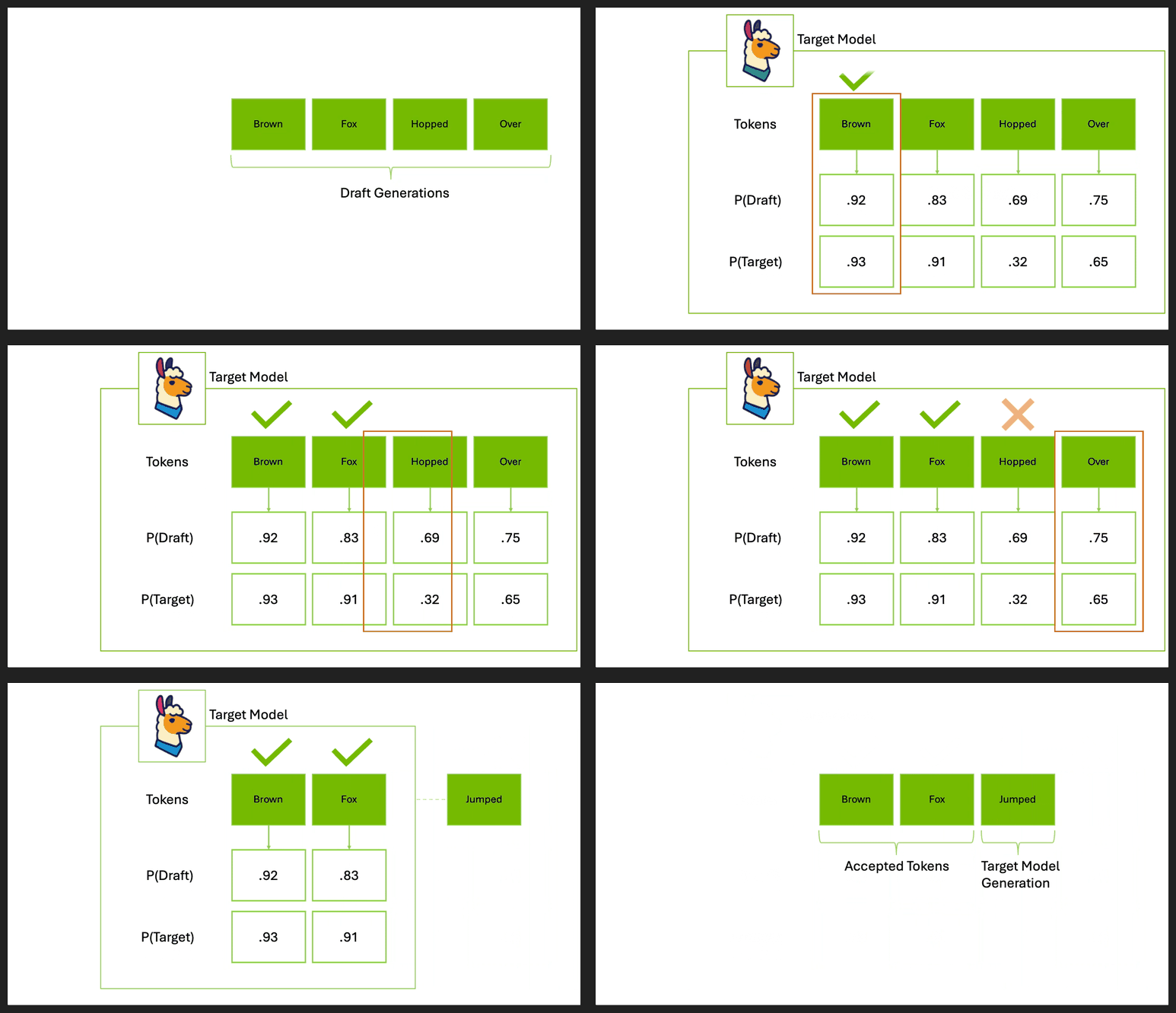
Let’s zoom in on this example a bit more. We have our four speculated tokens from the draft model, and we’re going to verify them with the target model.
Specifically, we’re going to check if the probability of the speculated token for the target model is at least as high as the probability of that token from the draft model. Like in our case, the target model thought “Brown” was 93% likely, and the draft model thought it was 92% likely, and since the target model is smarter, we take the increased probability as a sign that the draft model was pointing us in the right direction. Similar story for “Fox”.
But for “Hopped”, the draft model was more confident in that token than the target model was. That’s a bad sign and means we should reject the draft model’s choice.
Incidentally, when the target model rejects the third token, it substitutes its own - in this case it’s the word “jumped”. That extra token you get from the target model when it rejects the token from the draft model is called a “bonus token”, because you get it “for free” in the process of verification. If you’re really lucky and all your speculated tokens get approved, you get a bonus token after that, directly from the target model. Like if all four tokens had been right in this example, we also would have gotten a fifth token as well, with virtually no extra effort.
Now as you might imagine, the draft model is going to be better at predicting some tokens than others. Like on a hard reasoning problem, the acceptance rate will be quite low, maybe like 25%. But on a more structured and straightforward task, like using a web search tool, it could be near 100%. So speculative decoding isn’t a complete across-the-board speedup, but for a lot of mundane LLM uses it’s helpful. It’s really an empirical question depending on your use cases, your hardware, what model you’re using, stuff like that.
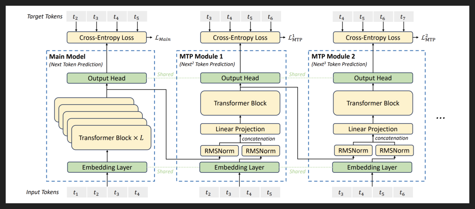
I should add that there are other forms of speculative decoding, or of trying to predict multiple tokens in one go anyway. We’ll briefly see one called EAGLE-3 in the paper for example.
Another example, which we’re looking at here, is literally called “multi-token prediction” or MTP. The difference with MTP is that is has to be part of a model’s training from the get-go, it’s not an external enhancement.
You can see it right there along the top, at the boxes labeled “Cross-Entropy Loss”. The loss is the single number that tells you how well your model is doing. In a normal model, your pretraining loss is based on how likely you predicted the actual next token in the training data would be. That’s the first box along the top, it has an arrow pointing to L_Main - that’s the symbol for loss.
But here in MTP, there are multiple losses! As you continue along the top, you’ll see L_MTP^1 and L_MTP^2 - the losses for predicting the first and second of the multiple tokens. So now your loss is from the normal token, the first MTP token, and the second MTP token. And if you do training right and minimize the overall loss, you can get pretty good at predicting multiple tokens.
Fittingly, modern MTP itself is an invention of the DeepSeek crew, although Meta invented the original version. Many other models now come with MTP. You can think of it as the baseline speculative decoding approach, which EAGLE-3 and DSpark and others must surpass in order to add value.
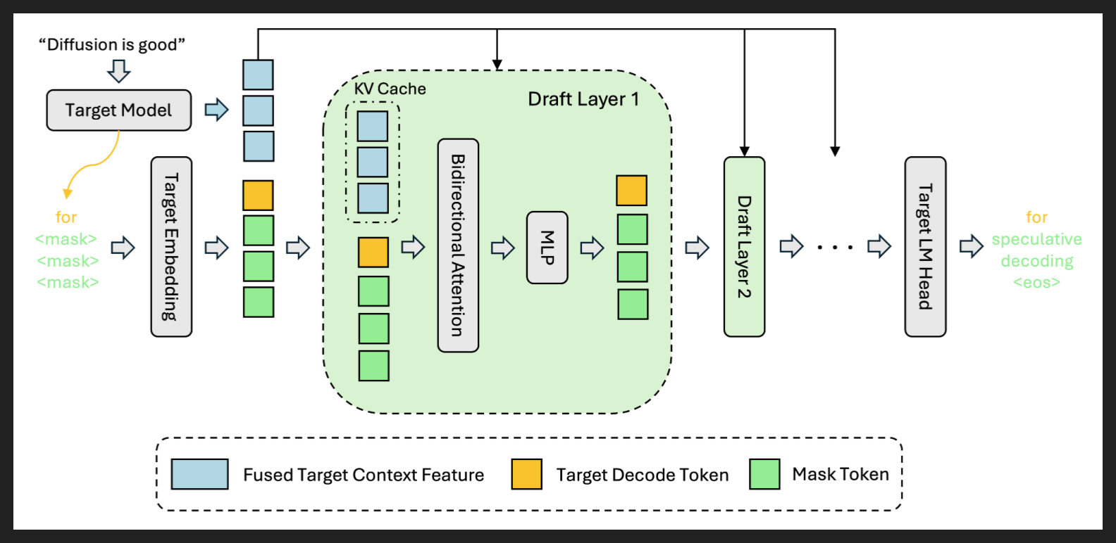
One type of speculative decoding setup is DFlash, pictured here. It uses the classic setup of a draft model speculating tokens for the target model to verify, not the MTP baseline we just saw. Like MTP before it, DFlash will serve as the base from which DeepSeek innovates, and may serve as the same springboard to popular deployment.
DFlash uses a diffusion-based model, which means it outputs multiple tokens in parallel. That’s actually what the “D” in the name stands for. By comparison, in a standard LLM you only output one token at a time. That’s called “autoregressive”. Even MTP is autoregressive, because the second speculated token depends on the first, and the third depends on the second, and so on.
Putting out tokens in parallel means faster prediction, which means faster throughput for your target + drafter system. However, predicting tokens in parallel usually leads to worse quality, since language is inherently serial, where the right next word depends heavily on what came before it. Like if two similarly likely predictions are “Of course” and “No problem”, then I might end up predicting “Of problem” or “No course” instead.
To me it’s kind of surprising that diffusion LLMs work at all! We’ll come back to how DFlash mitigates the quality loss in a minute.
So in this diagram, DFlash takes in one token from the target model and outputs three tokens in parallel - the green ones, which start life as the special token “<mask>” but end up as real predictions. Those green tokens at the end - “speculative”, “decoding”, and “<eos>” (a special token which stands for “end of sequence”) - are the speculative tokens that the target model will then verify. Again, pretty similar to the standard speculative decoding setup with an autoregressive draft model predicting three tokens out.
Even the guts of DFlash are similar. The draft model starts with an embeddings layer, which pretty much all models do, turning tokens into vectors that the model can work with. In fact the embeddings layer is from the target model directly, it’s not even part of the draft model. Then the two main layers - “bidirectional attention” and “MLP” - are much like the standard attention and feed-forward networks of a typical LLM. And the two layers together form a block, the dashed box in pale green, with multiple blocks in a row forming the bulk of the draft model. Then at the end there’s a language modeling head, exactly like in a typical LLM, that basically undoes the embedding and produces tokens again. That also is directly from the target model.
Now we come back to the twist that DFlash introduces to improve diffusion quality: the boxes in blue, which they call “Fused Target Context Features”. That’s a real mouthful, but all it means is they take some of the target model’s thoughts, or “hidden states”, and put them into the draft model’s brain at every block. That’s much faster than trying to feed all the previous output into the draft model, because the hidden states are already compressed and compact. It’s also higher quality, because the target model is much bigger and smarter than the draft model.
So now that the draft model can put itself more in the frame of mind of the target model, it can make better predictions. It still can fall prey to the perils of parallelism, like the “Of problem” example I gave before, but empirically it seems to do significantly better.
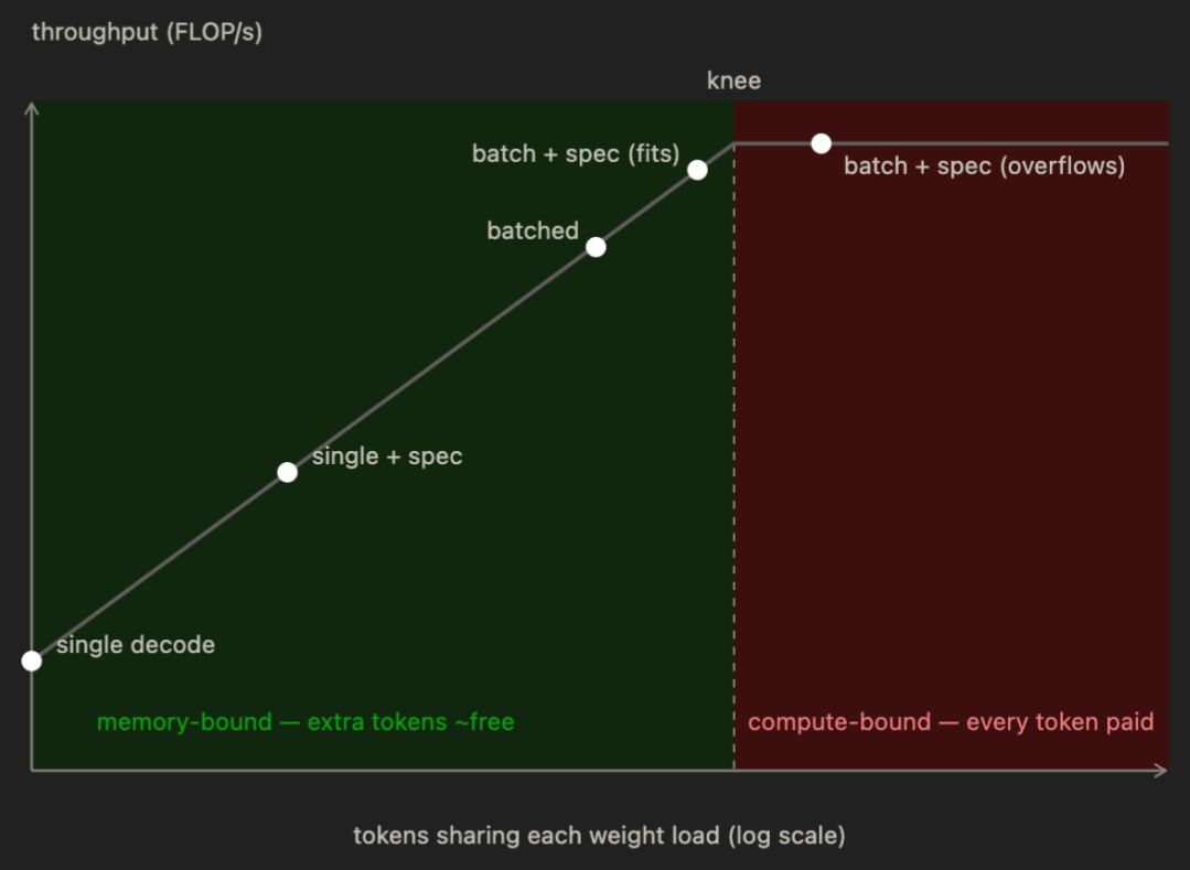
So this idea of speculative decoding, of adding this nearly-free verification step, depends on memory bandwidth being the bottleneck. Like if the weights from the current layer could just zap onto the chip, then the bottleneck would move back onto compute, onto how fast the chip could do the matrix multiplications to predict (or verify) the next tokens. You only get the “free” win of speculative decoding because you have this idle time waiting for the next weights to arrive.
But there actually is another way you could tip the balance from memory bandwidth to compute: adding more tokens for verification. Like if you tried to speculate and verify the next million tokens, you surely would spend more time verifying than you would waiting for the next layer to get to the chip. So somewhere between zero and a million there is a crossover point, where you’ve used up all the idle time with speculation.
In theory that’s the optimal spot: you have made use of otherwise-wasted compute availability, and you have not delayed the load of the next set of weights. Below that point, you’re leaving compute on the table. Above that point, you’re certainly not benefiting, and given speculative decoding is not accurate 100% of the time, realistically you are losing.
Now in practice a single user would never come anywhere close to this crossover point - you can’t realistically predict more than 10-ish tokens out at any likelihood of success. But for multiple users, in batch processing, it’s quite possible to overload the verification queue and slip past the crossover point, or “knee” as it’s sometimes called. And of course a big lab like DeepSeek is thinking about the batch case, because they’re serving tons of users and squeezing the hell out of every GPU.
So: we know we want to be right around the knee to maximize our compute throughput. What this doesn’t say is how to maximize token throughput, which will depend on maximizing compute throughput with the right balance of batch size and speculation size, but also on maximizing the accuracy of our speculation. And that is what DSpark is all about.
The Paper
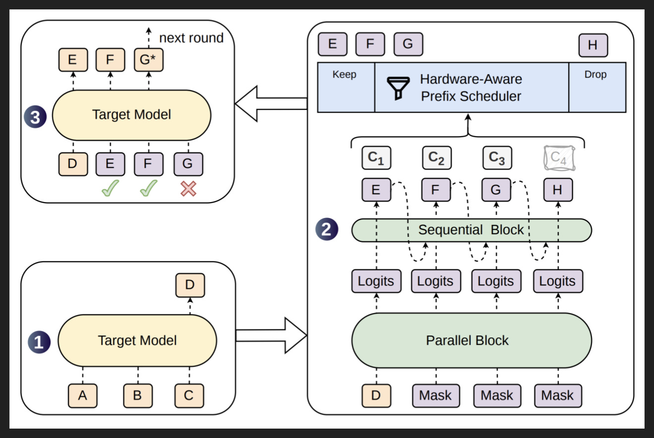
So this is the DSpark setup. We have our target model on the left, and our draft model on the right. The job of the draft model is to speculate tokens for the target to verify. In this case, given the most recent target model output “D”, the draft model will ultimately return tokens “E”, “F”, and “G”. The target model verifies E and F but not G, which the target replaces with the proper next token, “G*”. All totally standard.
What’s new is inside the big box on the right. We start with our parallel block, which contains between 1 and 5 draft layers, just like with DFlash. Each layer comprises attention and feed-forward, again like DFlash.
The two new additions happen after the parallel block produces its predictions, here called “Logits” because they are not tokens yet, they are distributions of token likelihoods. So going back to our parallel decode example from before with “Of course” and “No problem” colliding to become “Of problem”, the first position’s logits might say 70% odds for “Of” and 30% odds for “No”, while the second position’s logits might say 40% chance for “course” and 60% chance for “problem”. If we just take the most likely token for each position, we’re gonna end up with “Of problem”, which we want to avoid.
Since we have those probability distributions though, we still have the chance to tweak them to produce better outcomes. And that’s what this sequential block is all about. It’s a super lightweight way to add a little bit of sequential information to our otherwise parallel streams. So now for our second position, if we know we predicted 70% for “Of” and 30% for “No” for the first position, we can use that information and make “course” the more likely choice. That will add a tiny bit of time as we’ll see, but the accuracy gains will be worth it.
Now improved accuracy is always useful no matter the setting, but thinking back to our batch serving wrinkle, we also need the other new part: the grey boxes and the blue bar at the top.
The grey boxes are confidence scores, a score from 0-1 that DSpark assigns based on how likely it thinks the token is to be accepted. The blue bar, the scheduler, looks at how busy the GPU is and basically decides how big of a risk to take. Like if the GPU is super busy, then there’s not much idle compute between cycles of target model weights loading, so the confidence bar will be high and the speculation length will be short. Conversely, if the GPU is pretty free, then you might as well keep even the unlikely tokens in.
Remember, the parallel block generates the same number of tokens regardless, it doesn’t cost more to generate more at this scale. So the strategy is to generate a bunch, do a quick pass on which ones are likely good or not, and then filter from there based on capacity. In this example, apparently H was below the confidence threshold, so DSpark dropped it.
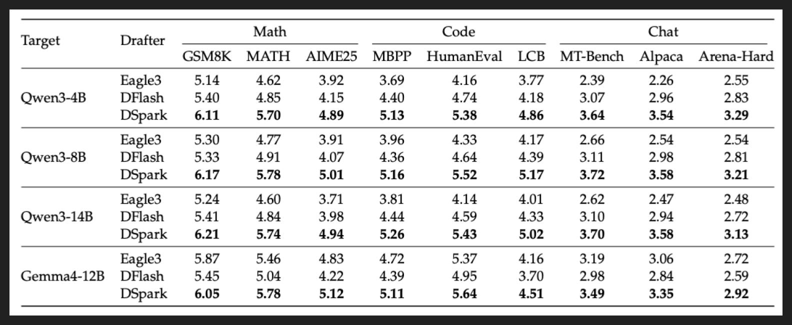
Now if we just focus on the first new feature, that sequential block that gives the parallel tokens a bit of information about the tokens before them, we can already see a big advantage in the average number of draft tokens accepted.
Across every benchmark and across all four models, DSpark is a strict improvement over DFlash, by about 10-20%. It’s also significantly better than another speculative decoding technique, Eagle3, that we will touch on a bit later.
One clear trend across benchmarks is the impact of domain on acceptance length. For math and code, which have more structure than natural language, the draft model can often predict pretty long sequences. By contrast, chats from a wide variety of users are often hard for the draft model to predict responses to.
Within the benchmarks, you can also see that easier prompts are easier for the draft model to predict responses to. Like GSM8K, which stands for “grade school math 8000”, is not hard even for small models nowadays. But AIME25, which is competitive math, is harder and thus less predictable.
So it seems the context greatly influences the risk-reward ratio for speculative decoding of all sorts. Hence the confidence scores! The DeepSeek folks love this trick of adding more learning in different parts of the model, like with mHC and Engram - two previous papers of theirs we’ve covered.
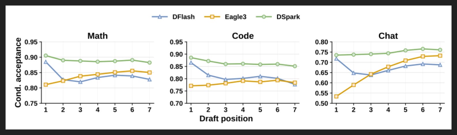
Here’s another way of comparing results across methods and domains. On the x axis is the position of the draft token, and on the y axis is how often that token was accepted, given all the other tokens before it were accepted. Because remember, as soon as one token in the draft sequence is rejected, the rest of the tokens after that in the sequence are discarded.
Before I explain the results, it’s important to remember that draft models have a hard latency cap, because they have to generate and send along their tokens in that bit of time where there is idle compute. So when we compare drafters, we expect roughly similar speeds.
However, we do not expect roughly similar sizes. That’s because for a given size, parallel models are much faster than autoregressive models. So if we hold speed constant instead, we expect parallel drafters to be much bigger. And bigger models are generally smarter.
That’s why DFlash, a parallel model, does so much better than EAGLE-3, an autoregressive model - at least at the start. Once you move past the first token though, DFlash starts to run into that “Of problem” issue, what the authors call “suffix decay”. The less structured the text, the worse the problem bites. That’s why the scores on Chat are lower overall, and why EAGLE-3 in particular rises so sharply. Remember though, this is all conditional on the prior tokens being approved, which on an absolute scale just gets less and less frequent the further you go in draft token position. So EAGLE-3 being better late-game doesn’t help as much as it might seem just from looking at these graphs - you have to keep the overall results from the previous slide in mind.
Anyway, that all is ultimately background for the DSpark results, which once again are superior across all domains and draft positions. That’s because DSpark blends the parallelism (and thus greater input context) of DFlash with the autoregression (and thus greater consistency) of traditional LLMs and methods like EAGLE-3. We haven’t even gotten to the hardware-aware part, which is novel.
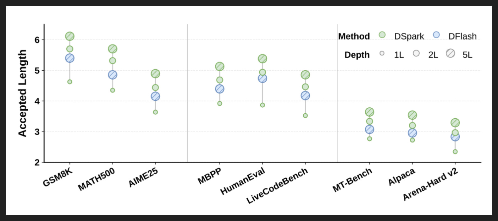
Now so far we’ve been measuring just one particular design of DSpark, when in reality there are two clear design knobs: the depth, i.e. the number of attention + feed-forward layers in the parallel block; and the block size, i.e. the number of tokens the parallel block predicts.
The previous results used five layers and seven for the block size. So now they’re gonna turn each knob a bit on both DSpark and its predecessor, DFlash, which has the same two knobs.
Although the layer knob isn’t even worth turning on DFlash, because DSpark with just two layers beats DFlash with five layers on every single benchmark. Five still improves performance and apparently fits the latency budget though, hence their choice in the previous slides.
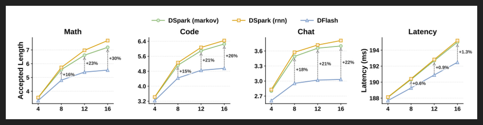
Now for the other knob, here they have fixed the layers at five but have moved the block size up and down.
Overall, greater block size there on the x axis does help, but the rate of improvement falls off quickly, especially above eight. On the negative side, latency increases directly with block size. You can see why they picked a compromise value, although it’s not clear to me why they settled on seven when they measured eight and when slightly higher values seem defensible. Maybe they had a maximum latency threshold and just picked the biggest block size under that? I’m not sure.
Also, I know there are two different DSpark trends on here, but the curves are so similar that it’s not worth getting into the difference between Markov vs RNN. It’s just two different ways of structuring the autoregressive part.
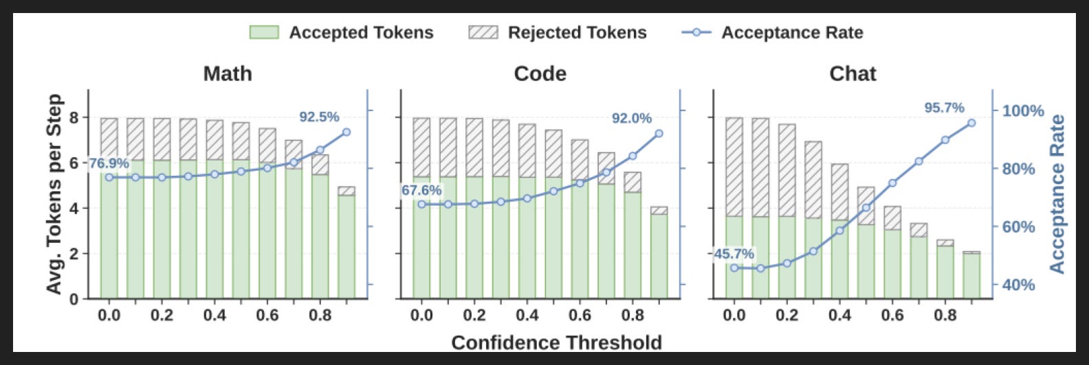
So far all the results have been hardware-agnostic, not taking the overall workload of the GPU into account. Now we can get into the hardware-aware part, which I think is the most DeepSeek-y aspect of the paper, given their reputation for squeezing every last bit of performance out of the limited hardware Chinese labs get access to.
As I mentioned at the top, DSpark looks at the available idle compute and decides how big a swing to take. If there’s lots of compute that would otherwise sit idle, DSpark takes bigger swings, since even low-likelihood bets could still end up with positive expected value. On the other end, if you have little or no spare compute - if you’re at or past the knee of that graph from the background slides - only a pretty likely sequence will have positive expected value, since you’re displacing a smaller number of guaranteed accurate tokens.
Now in general, confidence is going to decrease with token position, since it’s harder to guess tokens that are further out. But you could have some more predictable ones after actually. Like for a code problem, if the name of the function is somewhat arbitrary then the confidence may be low, but the parenthesis after it may be highly confident because that’s part of defining the function. So the way they deal with this is by calculating cumulative confidence when they do the cutoff, i.e. the confidences of each token up to the given position multiplied together. That guarantees the overall confidence is monotonic, it can only be flat or go down.
Anyway, as you’d expect, the higher the confidence threshold, the higher the acceptance rate but the lower the number of draft tokens DSpark gives to the target model for verification. The lowest confidence buckets in particular seem like free wins, basically no harm in cutting out those cases.
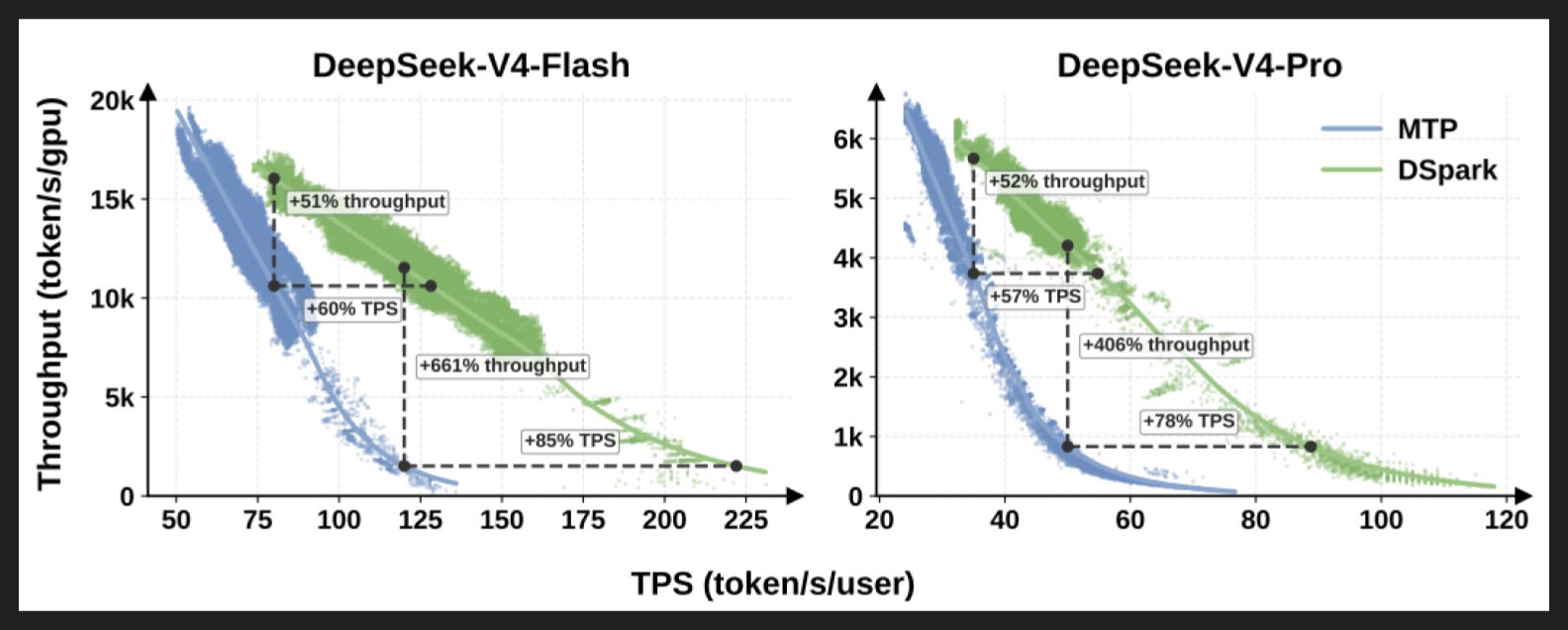
Here’s what I call the “money graph”. Not directly for the economic benefits of their efficiency gains, but because it really drives home how big a win a seemingly small change to DFlash made.
This is real production data from serving their current models. Each tiny dot is one combination of individual user speed vs overall GPU throughput. So they were able to collect a ton of empirical data on DSpark.
There are two ways to read this graph. One is at a trend level, where DSpark is clearly superior to MTP; the lines don’t overlap at all, and the gap is huge in some regimes.
The other is at a performance level, with one aspect fixed and the other one left to compare. That’s what the dotted lines are doing. So for example, with DeepSeek V4 Flash, if your GPU only needs to do about 1.5k tokens/second, then each individual user is going to see 85% faster throughput with DSpark compared to MTP. Or, starting from the same dot on the MTP trend - about 120 tok/s for each individual user - then your GPU can do 661% more tok/s overall. That’s crazy performance gain for practically no extra model size and latency!
My Takeaways
This seems like the right new default for speculative decoding
Just when MTP was getting popular!
Luckily, you can add DSpark to a model later on, whereas MTP has to be part of pretraining
I don’t think DSpark portends the triumph of full-blown diffusion LLMs (dLLMs)
Draft models don’t need to be that good to be useful
Perhaps standalone dLLMs will be useful for easy tasks where maximum speed is essential
Google calls DiffusionGemma “experimental”
Always learn where possible