


Originally presented as a live talk on September 23, 2026

Background

Ohh DeepSeek. DeepSeek DeepSeek DeepSeek.
Of course I was always going to cover this release. We’ve covered so many of your works before:
DeepSeek V4, the last major release from DeepSeek
mHC, a super technical improvement to a very specific part of the model architecture
Engram, a sort of built-in memory for common phrases
DSpark, a way to guess at upcoming tokens and thus speed up the generation process
You always have such wonderful tricks and such tough engineering. A researcher’s paradise! You charge next to nothing for your products and seem to care not a whit about commercial appeal.
Well you have, anyway. But things have changed for you in 2026, haven’t they? You sought your first outside funding. You were late for your V4 release - rumored to be before Chinese New Year but in fact released over two months afterward - and even then you called your release a “preview”. You arguably lost a technical bake-off against Moonshot AI, the makers of Kimi, with mHC vs Attention Residuals (linked above).
I don’t count you out. Nobody should. But it has been a rough year for you.
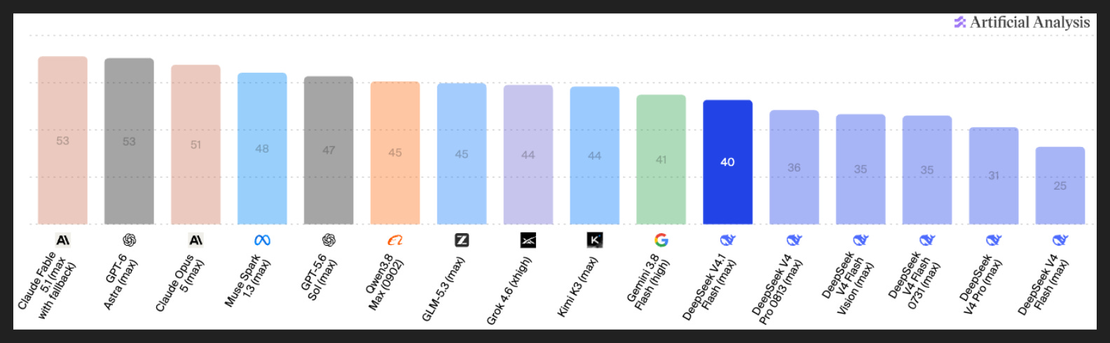
The Artificial Analysis Intelligence Index results here tell the story.
DeepSeek V4, both Flash and Pro, were underpowered. The vibe at the time was that both models had not gotten enough post-training, which sands down rough edges and really develops the finer capabilities. They are far behind the models of today, but even contemporary models had them beat. For example, Meta’s first Muse Spark model came out around the same time and slightly edged out DSV4P. For a new-ish lab playing catch-up to beat the most respected lab in China, with years of continuity and innovation, is both impressive for Meta and shameful for DeepSeek.
By this same measure, Qwen3.8 27B - which fits on a single prosumer GPU and is not on this chart - is clearly superior. 27B, compared to 10x that for Flash and over 50x that for Pro! Now that’s a bit unfair because Qwen3.8 came out four months later and is dense rather than MoE, but it is still shocking. Even if you look instead at the non-preview version of DSV4, the ones that came out in late July and early August when Qwen3.8 did, the capabilities of Qwen and DeepSeek are still on par.
4.1 Flash is more where we expect DeepSeek to be though, approaching the latest Gemini Flash release at least. Based on past trends we can expect a few points of improvement from Pro, which would place it nicely with its real competition like Kimi K3 and GLM-5.3 and Qwen3.8 Max - the other flagship releases from the other important Chinese labs. But they are at minimum late, and I feel like a disappointing release is a real possibility.
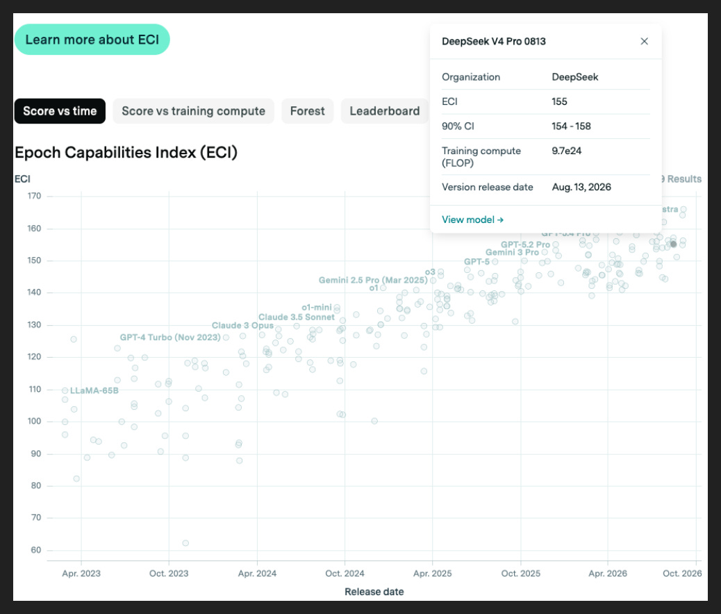
A couple other observations to situate DeepSeek further. One, their last flagship release is over six months behind the frontier as measured by ECI. Six months is the typical lag between the best American model and the best Chinese model, so they are once again behind the relative curve.
Now we don’t have an ECI score for DSV4.1F, but if you assume it’s one point ahead of DSV4P on here, then again, the leading American lab got there over six months ago - GPT5.3, back in February.
The other thing to point out is specifically how it does against Kimi K3, which I covered last week. As DeepSeek’s fortunes have fallen recently, Moonshot AI’s have risen, in sort of a mirror image. I encourage you to read that post after this one and judge for yourself. Anyway, Kimi K3 scored 158 on here, on par with GPT-5.4 Pro, and ahead of the six-month heuristic.
So DeepSeek has been in a bit of a hole in 2026. But DSV4.1F may be the first step out of it.
Speaking of trends, we have all witnessed the shift from chatbots to agents. And that trend has encompassed a lot of different things: the improvements in model intelligence and instruction following and tool calling and so on that allowed agents to work at all; the increase in context window size that made long trajectories feasible; the birth and development of harnesses for models to inhabit and thus become agents. Now it’s to the point where the primary use of a frontier model is as an agent, not really as a chatbot.
Which raises the question: what does an agents-first model look like?
Well for one, it should be able to handle a lot of input. With a chat-oriented model, typically the input will be small and the output will be large. Like if you’re a student asking questions about calculus, or you’re a grifter getting Claude to produce slop essays, you are providing a little context and letting the model spin its yarns.
By contrast, an agents-first model expects to receive tons of information. Not from the user - that won’t change much from chat - but from the environment. Any time your agent is reading the codebase or searching the web or analyzing documents, it is processing input and not yet producing tokens.
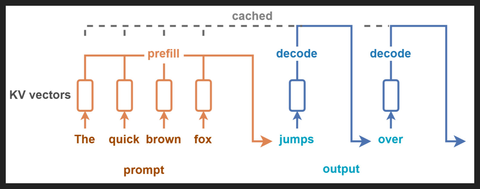
In the LLM lingo, we call that prefill and decode, respectively. Prefill happens in parallel, since we have all the input tokens available to us at once, but decode has to happen in serial, since we need to know the previous token before predicting the next one. Prefill and decode have different bottlenecks, on both the software and hardware side. Keep the software side in mind for when we get to the technical innovations.

The other important difference between chat and agent tasks is the density of information.
Again, consider a typical chatbot interaction. The user provides relatively little input on every turn, but the information that is there is almost always relevant. Prior model responses are also likely shorter and more consistently relevant. Humans can have long conversations but often many parts are germane.
Now consider a typical agent interaction. Let’s think about a research task, say, where the agent has to do a lot of web searches and trawl through documents to get the relevant information. The user input might be just as valuable, but a ton of the prior agent and environment output will not be. Like when you do research, you do a ton of Google searches of varying effect and may see tons of web pages or documents that don’t end up mattering at all. You only need a very fuzzy idea of what was in any of those traces. And if you did find something during any of them, there’s a good chance you wrote it down somewhere to collect or underlined it or somehow marked it out.
So when looking back at all the prior context, the agent does not need a thorough, rich understanding of all of it. What it needs is a clear view of a few key areas and a general notion of everything else.
So we have wildly varying levels of attention necessary, and we need to process inputs as quickly and cheaply as possible. That’s what our agents-first model needs to work like.
Now we already have existing DeepSeek work addressing both concerns. For attention, DSV4 introduced something called Compressed Sparse Attention (CSA). We are going to see a new version of that called CSA2 in this paper, so I am going to defer on CSA for now, but you can read about it in my DSV4 coverage.
As for processing inputs quickly and cheaply, the existing work is Engram, which I described earlier as a built-in memory for common phrases. Again, because we did a whole paper review on just Engram, I will refer curious readers to that installment.
There is a completely new aspect for DeepSeek related to processing inputs though, what they call Causal Encoder-Decoder (CED). And for that we need some new technical background. Specifically, we need to discuss the KV cache.
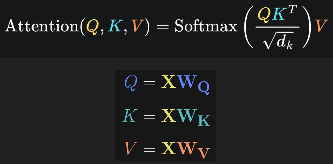
When you are using attention, you are taking your input X and making three different versions of it: the query (Q), the key (K), and the value (V). In the context of language, the query is like the subject of a sentence, the key is like the object of a sentence, and the value is the meaning of that subject-object relationship.
To understand a token as a query or as a key or as a value, you multiply it by the relevant weights (W), which the model supplies.
Now matrix multiplication, or matmul as the kids call it, is expensive. Really every operation is expensive at the scale of a SOTA model, but matmul is so core to the LLM and so frequent that if you can reuse previous matmuls, you should.
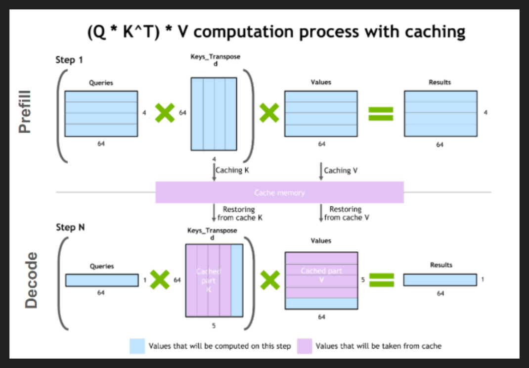
Now the standard way to save this compute comes from how prefill vs decode works. In prefill, all your input is new, so you have all this new matmul to do. Fine, you know it has to happen at least once for each token.
In decode though, you only have one new token to deal with at a time - the one you just produced. So there’s only one token that needs to be your “subject”, your query.
However, you still have to understand how this new token relates to every other past token. That means you need all the key and value versions of all the prior tokens. And you don’t want to recompute all that.
So when you’re computing the key and value of each token, you store the results. And those stored results are the KV cache.
Now a couple details to add to our picture. One, each attention layer has its own weights, and so it has its own KV cache. People talk about “the KV cache” as one giant pool, but really it’s more helpful to think of many KV caches, each associated with a particular attention layer.
Two, the KV cache is alterable, like any other part of the model. You can’t train the KV cache - it is ephemeral and only exists for a specific input, like your current state of mind - but you can learn how to do new stuff with it. It’s not just a common way to save compute.
By the way, you may have clocked that the KV cache grows along with your input. More specifically, it grows linearly with your input, in this baseline implementation anyway. Knocking that growth rate down is something all ML engineers shoot for, not just in this age of agents, and we’ll see a bit later how DeepSeek has managed to keep the KV cache relatively tiny.
The Paper
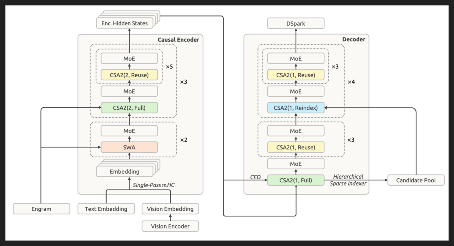
So this is DSV4.1F. It is kind of a lot to look at, with parts we need to explore in depth before the whole picture makes sense.
Now broadly speaking, we still have the foundations of any modern model: embeddings to turn input into vectors, attention to form an understanding of that input, and feed-forward networks to process that understanding. Here, the variously colored boxes are versions of attention, and MoE is by now the standard form of feed-forward network on flagship models.
There are a few new boxes and lines to point out though. On the left is our old friend Engram, which adds itself on to a couple carefully chosen attention layers. Remember, Engram is a cheap way to attach a lot of meaning to short phrases quickly.
Right between all the embedding boxes is mHC, DeepSeek’s tweak to the standard residuals. Then all the way at the end is DSpark, which speeds up output. Again, I refer you to the past presentations if you want to dig in more.
The main show is all about the attention layers and what goes into them. For that we need to note a few elements:
The notation: SWA is “sliding window attention”, a very common local form of attention that just looks at the most recent tokens before the given query. CSA2 is the real star, and it comes in various flavors, indicated in parentheses. The number indicates compression, so 1 means no compression and 2 means you compress two tokens into one. The word after it indicates the mode of CSA2: Full, Reindex, or Reuse. We’ll expand on that next slide when we dissect CSA2. We’ll also see that CSA2 includes SWA, meaning SWA is part of every attention layer. So we are always doing local attention, and most of the time we are also doing global attention. Just not at the start.
The left-right split: the authors divide the architecture in half, with the first half called the “causal encoder” and the second half called the “decoder”, hence the term “causal encoder-decoder” I mentioned earlier. I will get to what that all means in a minute. For now, note the even split: 20 layers of causal encoder, 20 layers of decoder.
The hidden states: the output of the causal encoder. A hidden state is just the output of a layer, so basically the output of the final layer in the causal encoder is going to have a special role in the decoder.
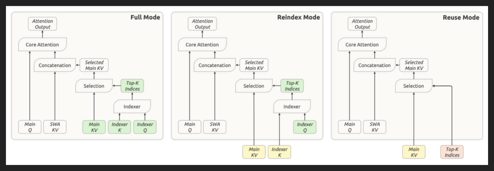
Okay, now we are ready to plunge into the guts of CSA2, which took me a long time to really get. So if some details escape you now in this review, I don’t blame you.
Now remember, the goal here is to do as little computation as possible while still achieving good quality. Everything is downstream of that efficiency goal, and that switch from chatbot to agentic use cases.
So the first thing to note is we have three versions of CSA2: Full, Reindex, and Reuse. They appear in order from most to least computationally intensive.
Another thing to note is how they overlap. Specifically, they all share the grey boxes in the Reuse Mode diagram. I will explain the steps in sequence, but use the Reuse Mode diagram to ground yourself as components of CSA2 change.
Last thing before we dive into the different modes is that we have two levels of attention: global and local. Global attention is normally more expensive because the cost of attention scales with how much there is to pay attention to; with local attention, you only look back at the most recent n tokens before your query token, in this case n = 128 for our sliding window. So all the fancy engineering to wring out efficiencies is gonna focus on global attention, which the researchers called “main” here. That’s why all the action is on the right side of each mode diagram, where your job is to select what from the main KV you want to combine with the SWA KV for when you finally do the attention calculation with the main Q.
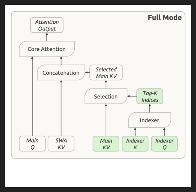
Let’s start with Full Mode.
Our inputs are:
Main KV, which we get by multiplying the input by the weights matrix W_KV. Note that in vanilla attention, we have W_K and W_V. Here we have only the one weights matrix, meaning K and V are always equal
Indexer K, which comes from Main KV
Indexer Q, has its own weights matrix to transform the input
Now for folks who came to the Kimi K3 session, you may recall that in the attention formula, Q and K multiply to produce the attention scores, which basically say how important each combination of any two tokens in the input is. That same principle is at work on the right when we run our indexer, taking these special versions of Q and K to say how important each position in our current input is.
Since we want to be efficient here, we’re only going to attend to the top echelon of indices for any particular query. In this paper, it’s 512. So even if you have hundreds of thousands of indices to choose from - because your input is in the hundreds of thousands of tokens - you gotta narrow down.
So you take your 512 top indices from the global context, from that main KV. Then you glue ‘em onto the SWA KV and do the normal attention operation.
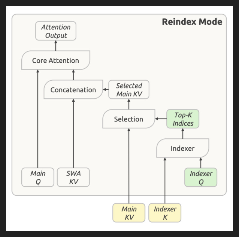
In Reindex Mode, we are doing almost the same thing. The difference is where our inputs come from.
Specifically, we reuse the Main KV and Indexer K from the most recent Full Mode CSA2 layer. So for global attention, this KV cache is not specific to this layer!
We do however need to compute a new Indexer Q. Otherwise we would be reusing all the information from Full Mode, so this layer wouldn’t be adding anything really. So the net effect is we take our same pool of index candidates but come out with a new top echelon, a new 512 we want to keep. Some computation saved, but much of it still left to do.
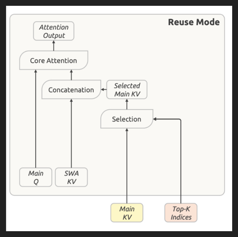
Finally we have Reuse Mode, which takes Main KV from the most recent Full Mode and the top echelon of indices from the most recent Full Mode or Reindex Mode. Reuse is the cheapest mode.
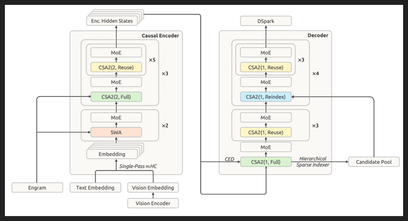
Now looking back at the overall architecture and where each CSA2 mode lands, we start to understand how they decided when to use each one.
The first two layers are SWA only, purely local attention. So the third layer, which is the first shot at global attention, has to be Full. Otherwise there is no Main KV or Indexer K to reuse.
After that comes five layers with Reuse Mode. To me that says, “we got a good picture of the global context already, so now let’s look at that picture from different perspectives”. Like the MoE layer right after the attention layer does some processing, so after that processing let’s reexamine our global picture with our new and altered local context. Because remember, we never reuse anything related to SWA.
Once you’ve done everything you can with that version of the global picture - after five blocks of CSA2 Reuse and then MoE - you form a new global picture. And you work with that, extract what you can, and do the Full + Reuse loop one more time. That is the Causal Encoder half.
Now note the Decoder half: there is only one CSA2 Full, and it’s right after the last Causal Encoder layer. So that is the last time you compute a new Main KV. And because of that, the Causal Encoder is the only part that runs during prefill! You only have to activate half your model when reading new input! That really puts all the savings at the individual layers into perspective.
So we have our now-familiar path of Full + a few Reuse. However, instead of cycling back to Full again, we do Reindex. Remember, Reindex is a different subset of the same global picture that Full drew from, it’s a different 512 indices to then stitch onto your local attention. But apparently it plays a pretty similar role to Full, where Reuse can draw new information from it a few times before you need to reshuffle again.
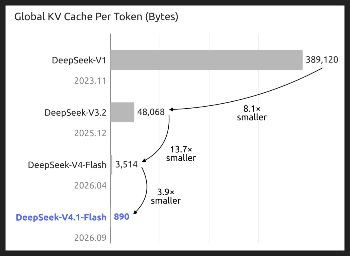
So that’s the mechanics, or at least part of it - there are additional details I left out for time. What’s the outcome?
Well one is a massive drop in the size of the KV cache per input token. Compared to the prior release, DSV4.1F drops it by nearly a factor of four. If you reach all the way back to the first release at the end of 2023, it’s a 437x drop! DeepSeek has been attacking this problem for a long time.
The upshot here is that the same hardware can support much longer trajectories, which is crucial in the age of agents.
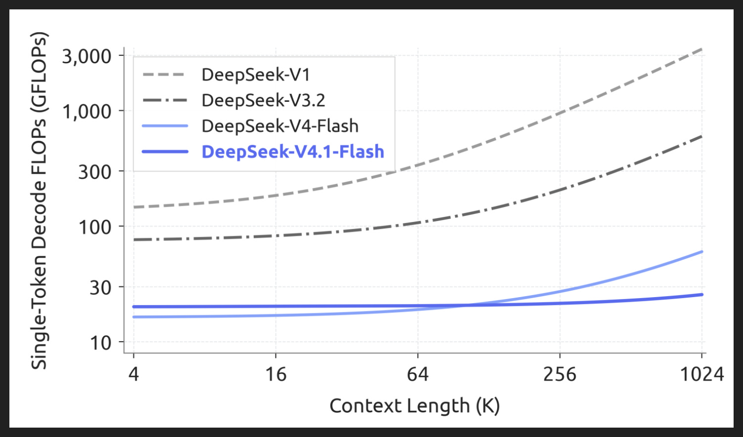
So we’re more efficient with our memory, but we’re also more efficient with our compute too.
To produce a new token requires a certain amount of compute, measured in FLOPs. And that amount of compute changes depending on how much context there is to look at and refer back to and consider.
DSV4.1 is actually a bit worse than its predecessor at smaller contexts - up to about 100k - but is barely sensitive to context length at all. Remember, this is a log graph, so what looks like a modest rise in the DSV4 trend actually matters quite a lot, and at long contexts decode speed is gonna drop substantially. For DSV4.1, decode speed would eventually drop, modestly.
Again, this wouldn’t matter so much for chat - it might even be worse - but for agents you are regularly gonna get into the hundreds of thousands of tokens on your trajectories, so the difference matters a lot.
Okay, so where does that all get us?
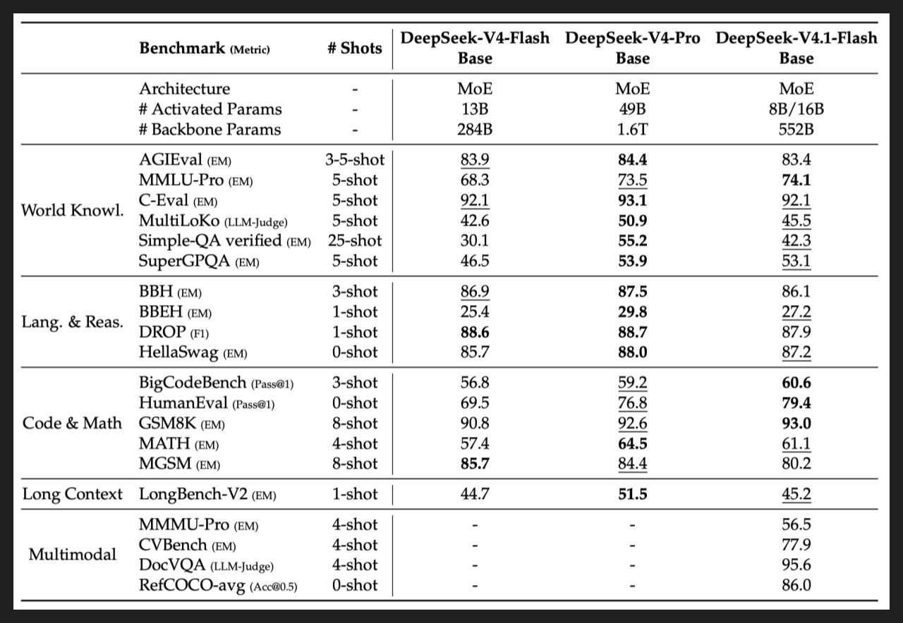
To answer that, let’s take a look at how DSV4.1F stacks up against both sizes of DSV4. We are going to look at base models, i.e. models that have completed pretraining but have not done post-training. Of course it makes sense to look at V4 compared to V4.1, but also, not many shops release base models anymore, so pickings are slim for this table anyway.
Also, before we look at the results, I want to call out the split in benchmarks. Pretraining is where the model gets all its raw information and its potential, which post-training then shapes. So you’ll see World Knowledge is the first section, and you’ll also see that the other benchmarks are mostly not that hard. It’s only later, after post-training, that models can do things like patch gnarly bugs or solve Olympiad-level math problems.
Now, the results. Despite having far fewer total and active parameters, DSV4.1F goes toe-to-toe with DSV4P. And actually, if you judge on parameter count, you should really think of Flash as closer to 400B; the Engram portion, which is more like a lookup table, is 196B parameters, so if you discount them heavily that 552B total drops substantially.
Anyway, Pro is probably better based on some vibe checks I’ve heard as opposed to just benchmarks, but it’s at least close, which is impressive. I’m not surprised to see Pro generally in the lead on the World Knowledge benchmarks, since knowledge tends to correspond to total parameters, but Flash leading on some Code & Math ones is impressive.
To be fair, DSV4.1F got about 39T tokens of text in pretraining compared to 33T for DSV4P, but I don’t think 6T more tokens of pretraining would have closed the Flash-Pro gap for V4 - some of it has to be down to the architecture.
As for what’s in that pretraining data, they don’t say much, other than the standard stuff about improving quality and removing duplicates etc. The one interesting detail for Scale is “we involve more domain experts to construct fine-grained data quality evaluation dimensions”, which maybe is like rubrics for pretraining data? Hard to say exactly.
Now let’s move on to post-training. As is standard nowadays, the researchers conduct SFT on one checkpoint, then RL on several checkpoints to create teacher models, then do multi-teacher on-policy distillation (MOPD) to create the final model. In fact, they call this the “standard paradigm” and explicitly avoid innovation here, focusing exclusively on the data. Here’s a direct quote:
“We find that, under a fixed and unremarkable optimization procedure, systematic improvements in the scale, diversity, and verifiability of synthesized data and environments account for essentially all of the observed gains.”
So because they want to lean on their own model to generate training data, they start by training the model to create better training data. Each task consists of a problem, an environment, and a verification system. They evaluate generated tasks based on difficulty and correctness, although they don’t explain how. They also watch the traces when the generated tasks actually do make it into the RL pipeline, to gather real-world evidence about quality.
Speaking of real-world data, they mention collecting traces and feedback from internal and external users on a voluntary basis. They use the traces to reconstruct environments, mocking popular SaaS apps but also proprietary software and backend systems. They focus in particular on recreating failures observed and reported in the wild, targeting them for improvement.
For coding agent data in particular, they describe a multi-agent process for turning popular GitHub repos into environments. Again it’s high-level enough to be nothing revelatory - one agent makes sure the repo actually can work in a container, another scrubs it for information that could leak answers, stuff like that - but I thought it was interesting that DeepSeek landed on the same generalist-coding split that Moonshot did in thinking about agent training and capabilities.
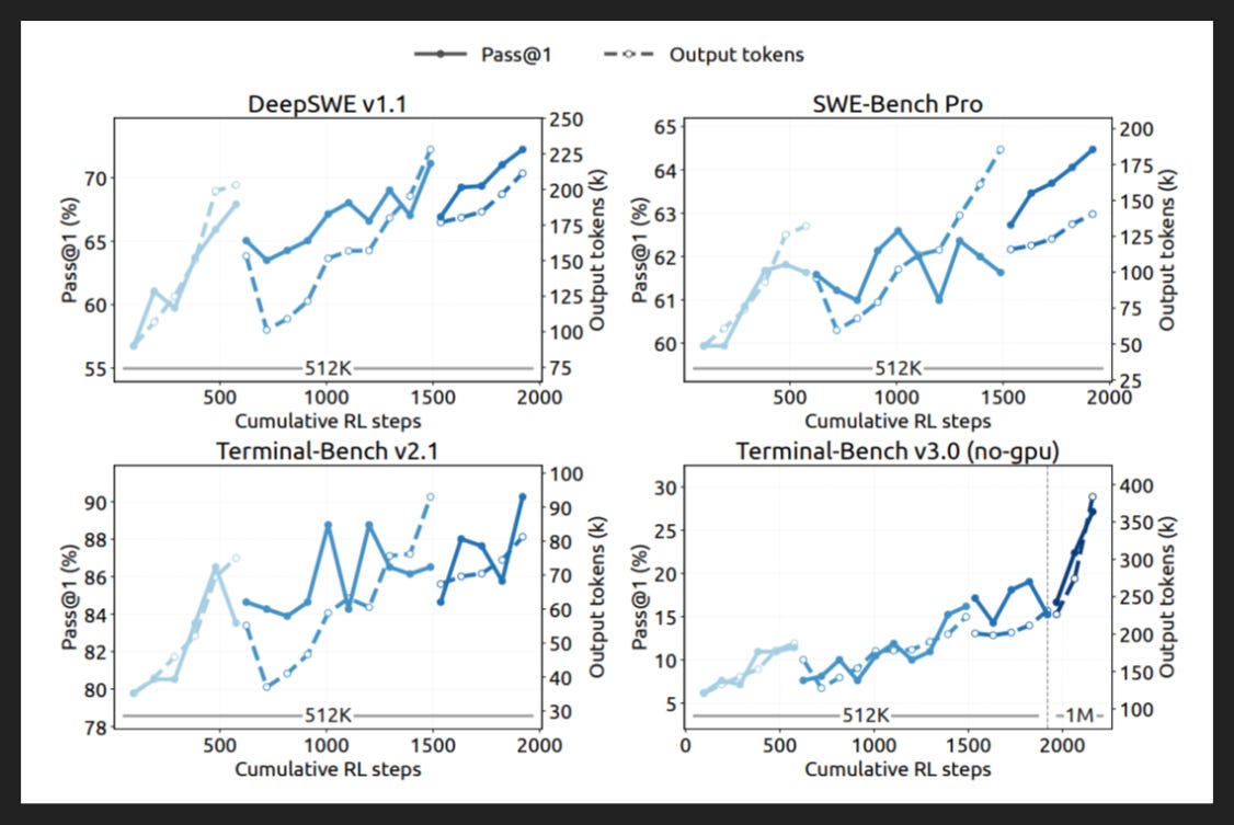
Of course coding is where the big money is these days, and is also how labs plan to hit recursive self-improvement, so it comes front and center. Here are some RL runs on popular coding benchmarks. The discontinuities and changes in color indicate model reinitialization, basically taking concurrent RL runs with different harnesses or configurations and merging them after a certain number of RL steps. So like let’s say you start with one checkpoint and make one copy each to put in Claude Code, OpenCode, Pi, and DeepSeek Harness. You train your four copies, they all become somewhat different, then you merge them to smooth out the idiosyncrasies while hopefully keeping the real gains.
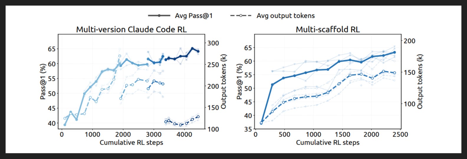
Speaking of harnesses, here’s a look at what impact they can have during RL.
On the left we have several curves for different versions of Claude Code. It’s a bit hard to see the lighter shades, but overall the trend lines for both pass rate and output length pretty well overlap. Also I’m impressed to see how the final run in dark blue cut trajectory length almost in half.
On the right we have trends for various scaffolds, including OpenCode, Pi, and DeepSeek Harness. Again, some variation but pretty similar trends.
My hunch is that because benchmarks are supposed to be diverse, you get a sort of averaging effect and any reasonable harness is about the same as any other. But in the real world, where you mainly work on one or perhaps a few projects and you have your own ways of working and so on, individual users feel a big difference on harness sometimes. That’s how I would reconcile the frequent reports of big differences in harness against this apparent similarity between harnesses.
To be fair, they do have a table later showing a nine-point spread on one benchmark depending on the harness, but with error bars around each score I don’t think it’s a big deal.
I also think Anthropic and OpenAI in particular don’t want good performance outside of their own harnesses, similar to how Apple software only works with Apple hardware and functions more as a whole than as separate components. So if folks are using Claude or GPT in OpenCode for example, and they have prior experience in Claude Code or Codex, that would explain the disappointment. The open-weights model companies on the other hand do want good performance on popular harnesses, since their models can crop up anywhere and be part of any stack.
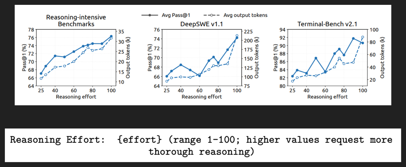
One other fun detail from their RL training is how they added reasoning effort.
By now the user-facing terminology is basically settled: low, medium, high, xhigh, max. Not everyone has every level, but reasoning effort is a thing and users expect it to look like that.
Under the hood though, it’s not obvious how you would get the model to actually obey, and from what I’ve seen different labs do it different ways.
For this model, the DeepSeek folks decided effort would be part of the system prompt (during training and inference) as shown here: a number from 1-100. 50 means “low”, 75 means “high”, 100 means “max”. For API users you can only pick from those three, but if you’re hosting yourself you can plug in any number you want. Heck, you could even put in some nonsense value or delete it from the system prompt entirely!
It’s not just the instruction in the text that controls effort during training though. They describe how the numerical value for effort feeds into a length penalty formula, which is how the model learns what effort really means. So it’s no surprise that effort tracks output token length more than pass rate. The jump in output tokens for max reasoning effort is particularly notable, like the model is tracking down every possibility no matter how remote.
I kind of wonder if the lower scores are just the model sandbagging a bit. Like if you told me to put in a low amount of effort, I might know what the right thing to do is but take the easy option instead and pretty much know it’s gonna turn out wrong. I know what they’re actually controlling is token output length, but there is clearly some connection between effort and outcome. Maybe that’s why they didn’t test at values below 25 and why in the API you can’t get a value below 50.
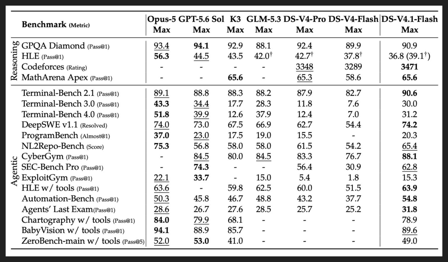
Now we can finally check out the final model’s benchmark scores. Notice how dominant agentic benchmarks are, and how the first nine in the list are about code.
The competition here is also instructive. They are going up against Opus and Sol, not Fable. (Astra wasn’t available at the time.) It’s still impressive that what’s likely a Sonnet/Terra-sized model can go up against Opus/Sol, but in real usage I do not see folks abandoning Anthropic and OpenAI for DeepSeek.
It’s getting harder and harder to measure model quality with benchmarks, both because of the more subtle and subjective differences and because benchmarks are saturating so quickly. Just look at the jump on some newer benchmarks from DSV4P to DSV4.1F: almost 20 points on Terminal-Bench 3.0 and Terminal-Bench 4.0, 10 points on DeepSWE, 10 points on ExploitGym. Those benchmarks are all only a few months old.
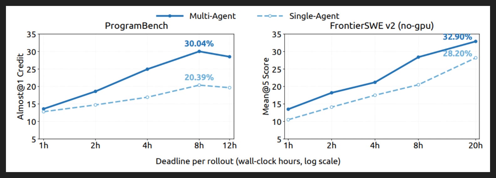
One area that doesn’t get enough benchmark love, and where I was disappointed by the Kimi K3 paper, is multi-agent.
There are some fun details in here about how they structured the swarms. The harness lets the lead agent create teammates, assign them roles, and pick what context they start out with. There’s also a “peer mailbox”, kinda like a group text thread or Slack, plus a kanban-type board for tasks. The lead agent monitors and can interrupt any other agent.
As for training, they add a collaboration bonus to encourage teamwork and a latency penalty that encourages parallelism and discourages synchronization. I would love to know more about how they came to their design and how it may have evolved, but alas, they give only the current state.
Now neither benchmark here is multi-agent per se, but it’s instructive to compare solving the tasks with one vs many agents.
In theory there can be a quality benefit from multi-agent, along the lines of specialization and swim lanes and clean context, but of course we all know how badly group projects can go. So solve rate is going to be an empirical matter. However, multi-agent should pretty much always win on time, on how long it takes to complete a task or how much progress can happen in a fixed amount of time.
What we see here is a bit of both, and somewhat different stories. On the left, I see mostly the story I expect, where multi-agent isn’t any better initially but opens up a wider and wider gap over time as the benefits of parallelization accrue. The dip at the end is unexpected, although it happened for both cases.
On the right though, I’m surprised that multi-agent starts off better yet doesn’t increase its lead almost at all. So maybe the tasks have a lot of dependencies and can’t really become very parallel. The mythical man-month and all that.
By the way, if you’re looking at the ProgramBench results and wondering what “Almost@1” means: it’s a slightly easier threshold for completeness, specifically that the solution passed at least 95% of unit tests.
My Takeaways
DeepSeek is still in the fight
I’m optimistic about DeepSeek Harness, but I’ve heard it’s not quite there yet
They don’t make it easy for themselves when they give away so much research! Qwen has already incorporated Engram for example
LLMs are becoming inscrutable
So many fine details
RSI will accelerate this process
We will deal with this by adding a layer of abstraction on top, which is how we deal with all systems that become too complicated to understand wholly on a certain level
Still lots to do with multi-agent
Hasn’t trickled down to training data or architecture etc
I expect team design (and eventually team self-improvement) to get just as much attention as harness design
Already quite relevant due to the Hugging Face incident and similar swarm actions