


Originally presented as a live talk on November 19, 2025

Background
To understand this paper at all we have to understand the main bit of jargon in the title: Monte Carlo Tree Search, or MCTS. And to do that we will break the term down into its constituent parts: Monte Carlo, and Tree Search.
So, Monte Carlo method, what is it? Well as the name implies, Monte Carlo originally being the name of a casino in Monaco, it’s all about chance. Specifically, how you can use random tries over and over again to get a pretty good empirical idea of something that you’re having trouble calculating theoretically.
Let’s say you’re an ancient Egyptian and you want to know how to calculate the area of a circle. You’ve worked out that it’s proportional to the radius squared, but also some other number, some constant you can’t pin down or derive purely mathematically. What do you do?
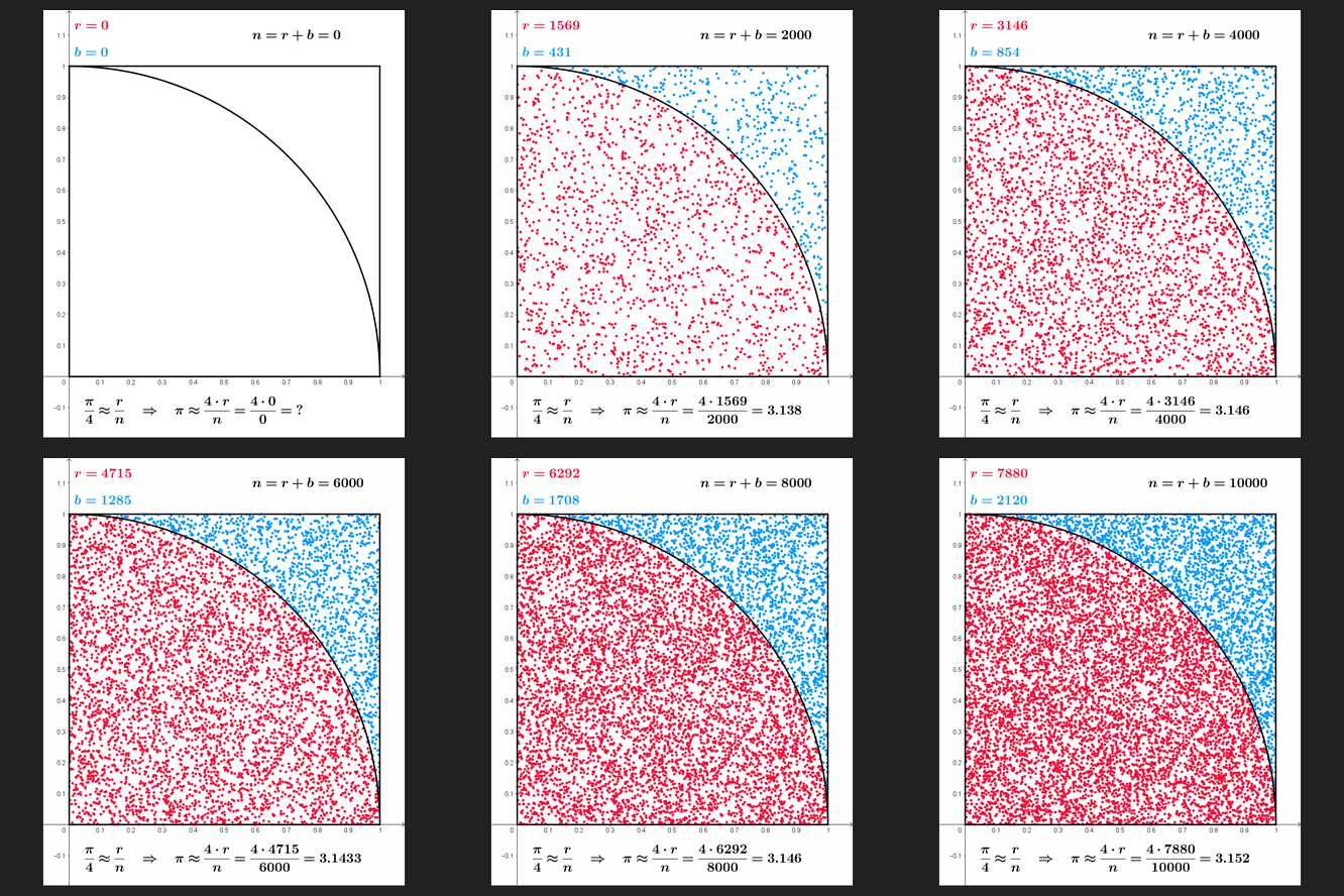
Well you can try getting a pretty close estimate by drawing this shape: a square with side length 1, and a quarter of a circle with radius 1 inside. The area of the square is 1 - that’s easy - and the area of the circle is pi over 4, since the full circle is pi-r-squared and r is 1, which means the full circle’s area is just pi, so the quarter circle’s area is pi over 4.
And that means the ratio of areas is pi over 4, over 1, so just pi over 4. So if you can empirically find that ratio of the inscribed area to the whole area, the quarter circle part to the whole square, then just multiply by 4 and you’ll have pi.
The way you empirically find that ratio is shown here. If I’m that ancient Egyptian and I’ve drawn this pattern on some papyrus or whatever, then I can get a little pebble or something and drop it from some height and mark where it lands, over and over and over. Then I just take the number of marks in the circle and divide it by the total number of marks. The more random marks I make, the better my estimate of pi.
Now this is a toy example of course because we have far more precise ways of calculating pi. But in real life there are many cases where the theoretical calculation is impractical, impossible, or not even known yet. So Monte Carlo is still a popular method.
So that’s the Monte Carlo part. Now we need the Tree Search.
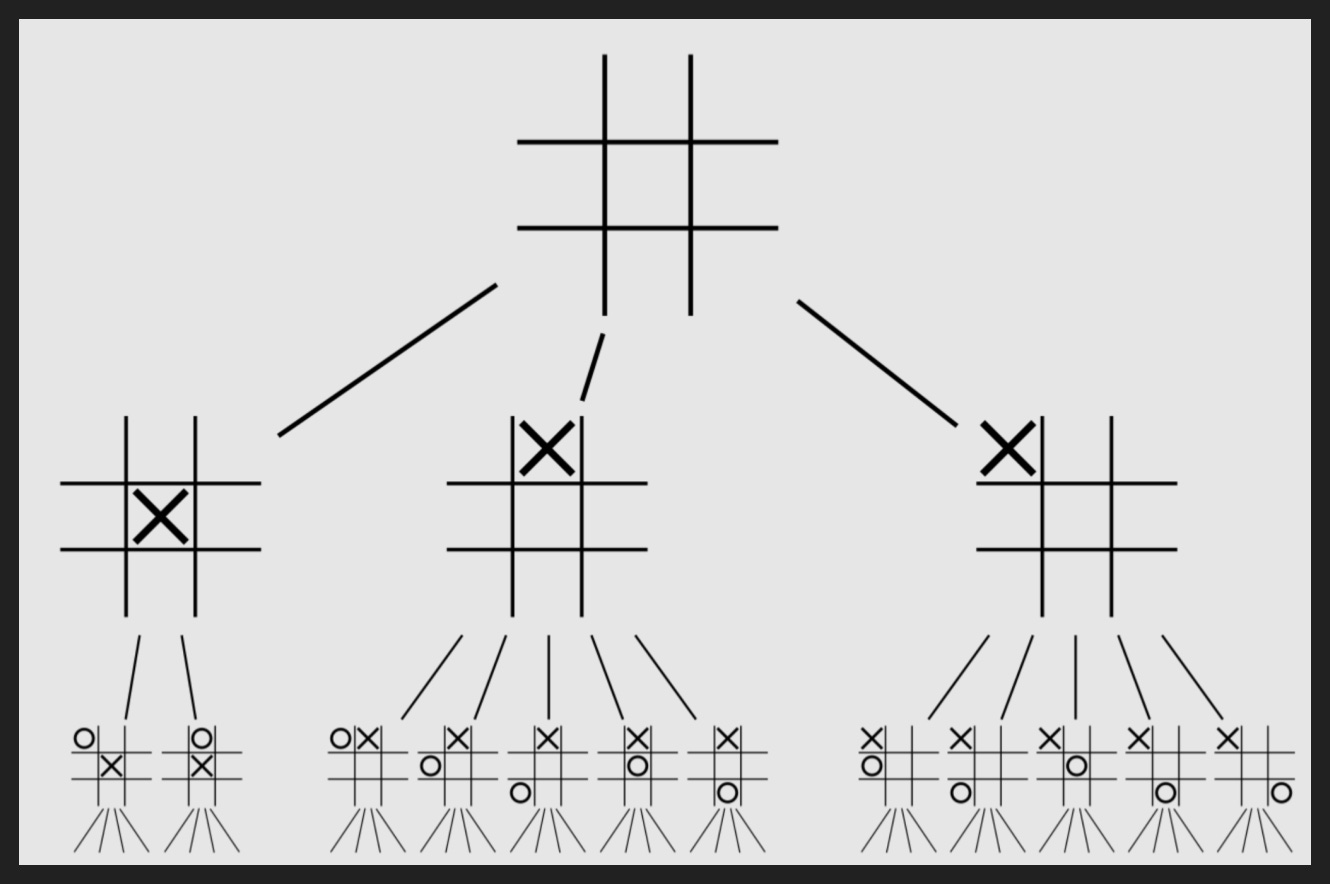
To explain this I’m going to use another toy example, this time Tic Tac Toe. What we see here is the different possible states of the board, starting from blank and progressively covering every possible state until someone wins or there’s a draw, although this one only shows three levels deep. Also if you’re wondering why some versions are missing, it’s because we group cases that are the same if you flip or rotate them. So like the last board in the second row, with the X in the top-left corner, that covers any board with just X in one corner.
This structure is a tree, specifically a game tree. The search part isn’t really relevant since this is such a simple example and we can analyze every possible game state pretty easily.
But imagine a much bigger game like chess or Go, where drawing a game tree is theoretically possible but practically impossible. Or something even crazier like language or math, where again you could in theory map out every single choice of next word or character to produce, but practically it would be impossible.
What you need is some heuristic, some way to decide which nodes in the next layer are actually worth diagramming out so to speak, which next steps are most promising.
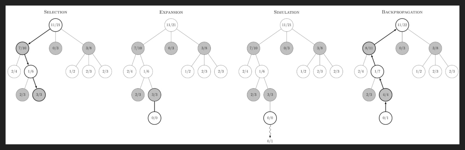
Enter Monte Carlo Tree Search: a method for expanding that tree in the most promising directions. This diagram explains it using a game between a white side and a black side, like chess, where the white circles are moves the white pieces can make and the black circles are moves the black pieces can make.
There are four steps:
Selection: start from the beginning, make reasonable choices along the nodes you’ve already mapped, until you reach the bottom of the existing tree - not the end of the game or the response or whatever you’re searching, otherwise there’d be nothing left to do with that node. In this example they’re always picking the lowest win ratio for white and the highest win ratio for black, which is the simplest method but isn’t optimal for finding the absolute best path - too much exploitation and not enough exploration, in the ML lingo. That’s why I said “reasonable choices” earlier.
Expansion: again, assuming this is not a terminal node, map out the next moves you can make. In this example there is apparently only one, which is plausible for a simple game, but for a complex game or in other domains, there will always be many possible choices. Anyway, the win ratio here is currently 0/0 because we haven’t done anything forward-looking with this new node yet.
Simulation: this is the tricky part. You have to have some way of estimating the value of picking this option. The standard, simplest way to do that is to keep playing from that point forward with random choices, until you reach an end state. Then you report back what happened. In this case, apparently black won and white lost in this random simulation, so since this is a white node we report back a loss and update the win ratio to 0/1. Now this probably seems silly - surely both players making random moves is not actually how any game would play out - but that’s the insight of the Monte Carlo method! If we do this loop over and over again, the randomness of any one simulation won’t matter, it’s the collection of all the random simulations that paints an increasingly accurate picture.
Backpropagation: now that you have more information about this option you’ve just created, you also need to let all the other, earlier options know what lies in their future. Note that the white circles have added a loss, but the black circles have added a win - the 1/6 for white went to 1/7, the 3/3 for black went to 4/4, etc. Updates all the way up the tree, that’s backpropagation.
There are many complications and variations on MCTS, but now you understand the basic idea of looking at the most promising path, picking a next step, doing a random trial for all its future steps, and updating the path based on that trial.
Now what does this all have to do with AI? Well first, MCTS is behind a lot of the AIs used to master increasingly complex games. For example AlphaGo, which handily beat the world champion of Go in 2016.
But second, MCTS was one of the techniques rumored to power o1, the first reasoning model and a major breakthrough in LLMs from OpenAI.
If you were following the rumors at the time, you may remember the name Q*. Right around the time the OpenAI board briefly fired Sam Altman, some OpenAI researchers had sent a letter to the board warning about an internal project called Q* that was unlocking significant milestones in math and reasoning. Ilya Sutskever - a cofounder, board member, and chief scientist at OpenAI - was leading the Q* project. People started wondering if Ilya believed OpenAI had dangerously advanced AI on its hands but that Sam was disregarding safety in the name of progress.
As we know now in November 2025, based on depositions released last month, Sam’s firing and Q* were unrelated. But the drama of Q* got people speculating about what it was under the hood. The name seemingly came from Q-learning, one of the many RL algorithms, and the A* search algorithm. That combination of planning and search is just like MCTS.
Anyway, later in summer 2024 we started hearing about Project Strawberry, again a supposedly super advanced model from OpenAI. This time Sam Altman played into the hype, posting photos of strawberries and engaging with a mysterious Twitter user with strawberry emojis in their username saying “welcome to level two”, a reference to a reasoning-related milestone on OpenAI’s path to AGI.
Again, people speculated that this new model used a planning + search method like MCTS to iteratively find the correct reasoning path. But now with o1 and its successors released, when looking at the chain of thought it doesn’t seem like they’re doing something so systematic. It’s more like thinking longer, maybe checking assumptions, much more organic stuff than building a search tree methodically.
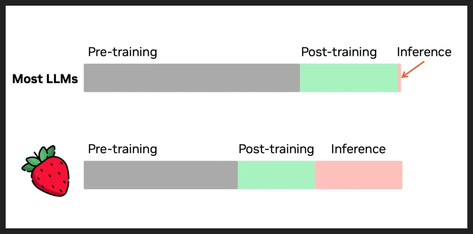
This chart lays out the main advance of o1: using a lot more tokens to “think” before giving a final answer. And as the official blog post from OpenAI showed, the longer you got the model to think - the more inference you did - the better your performance got. Nowadays people call this inference-time compute scaling or test-time compute scaling.
So o1 came out in September 2024, but for the rest of the year nobody else released anything like it, and we of course got no publication or confirmation from OpenAI on the techniques they used to make this so-called “reasoning model”.
Then came the DeepSeek moment: the release of R1 in January 2025.
The Chinese lab DeepSeek, which had been quietly building increasingly capable models, dropped the weights and an accompanying research paper for their own reasoning model, R1. In the paper, they revealed reasoning did not require fancy planning + search algorithms; instead, it was plain ol’ RL, specifically RLVR, rewarding the model whenever it got math problems right. No principled method for planning and searching, just trial and error over and over and the magic of RL.
Now the DeepSeek team also released their particular RL algorithm, GRPO, which is a simplified version of PPO, and that definitely helped simplify and stabilize training. But the key insight was RLVR.
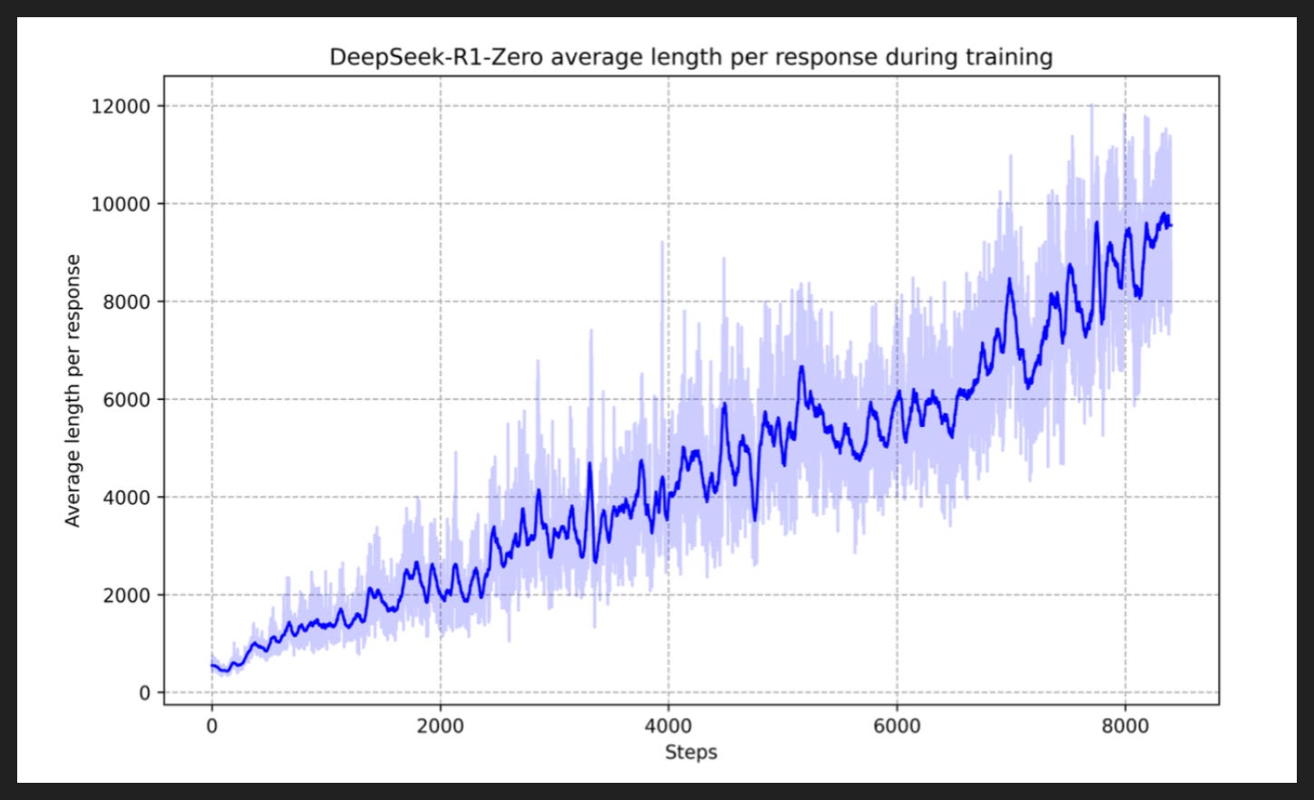
This chart is from that R1 paper, showing how the response length - the amount of reasoning, the amount of inference-time compute - grows and grows the more you train the model on their setup.
This big reveal from DeepSeek really took the air out of MCTS research for LLMs. We got a flood of o1 imitators after R1 broke things open, and all attention turned to RLVR. At least until now.
The Paper
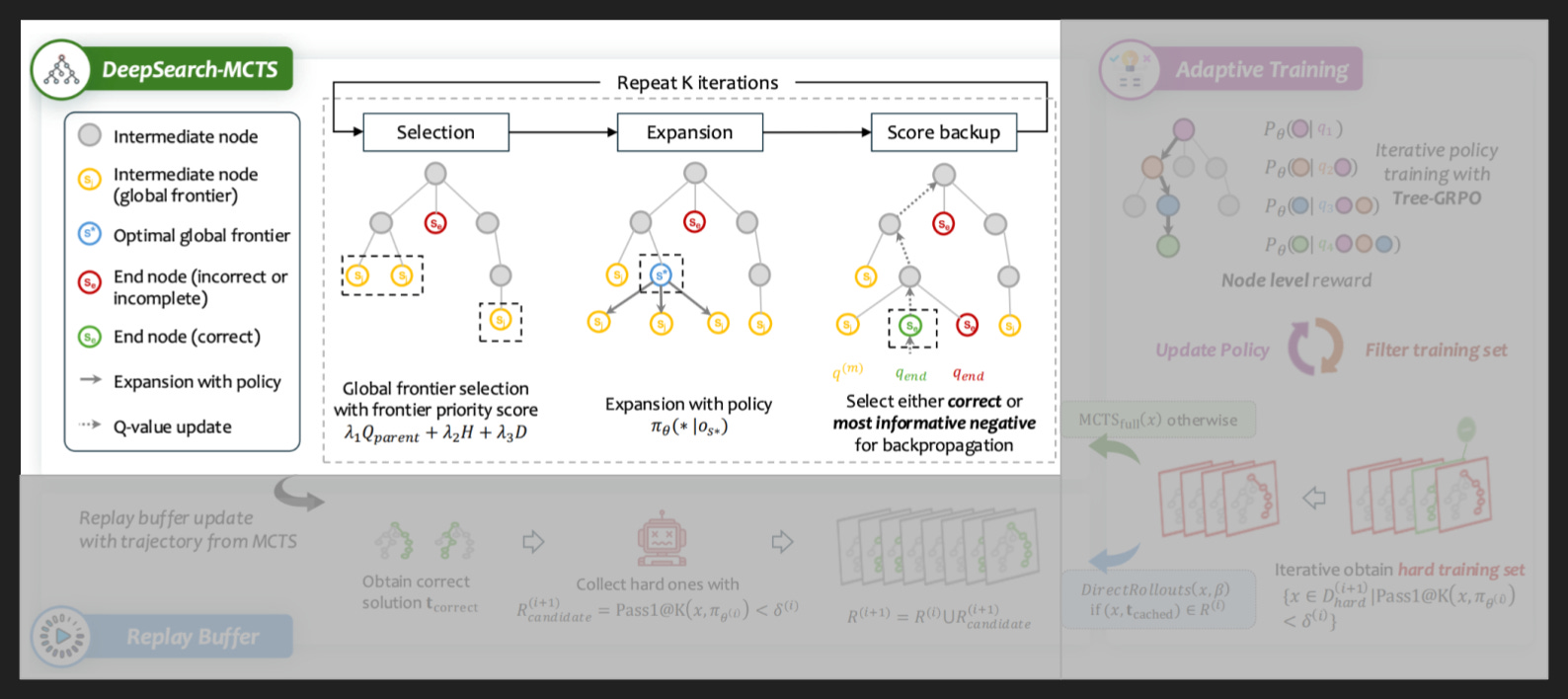
Okay, this is going to take some serious explaining even with that background.
The first bit is of course the MCTS. They do a loop similar to the one we saw before, but there’s no simulation step where they take one node and make something like random choices until they hit a terminal state. Instead, if all the nodes in the expansion step are intermediate rather than terminal, they go back to the selection step.
So when you finally do get a terminal node, you send that information back up the tree like in the backpropagation from normal MCTS. A node has a higher score the more correct paths it’s involved in and the closer it is to the correct node. Of course some nodes can be on the path to both good and bad outcomes, but if it’s on the path to a good outcome then they guarantee the score will be at least a little positive.
Now I did want to say one thing about the selection step. They have this “frontier priority score” thing that looks mysterious on here but which they explain in the text. Basically they’re picking nodes to expand with three aspects in mind:
The quality potential, which looks at the quality score of parent nodes. That’s Q_parent
The uncertainty, as measured by the entropy, which rewards nodes where the model is less certain and therefore more exploratory. That’s H, the traditional abbreviation for entropy
The depth, as in how many nodes down it is, which tends to mean you’re closer to a terminal node. That’s D
So the heuristic here is: the earlier steps in the reasoning chain should be good, and the next step we choose should be somewhat uncertain so that we can look at a few different paths and learn which one is the best. But we also don’t want to just keep making intermediate steps forever and never get to a solution.
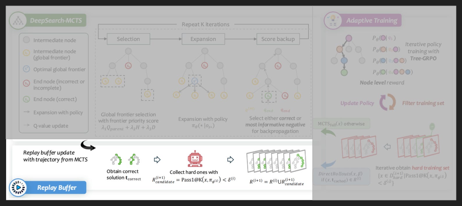
The next bit is this “replay buffer”, which collects the correct reasoning paths the model has found with MCTS.
The only tricky bit is the middle step with the red robot. The notation is dense, but all it’s saying is we only want to keep training on solutions the model is unlikely to get on its own. If you keep training on problems you already get right then at best it’s wasted effort but at worst you start to memorize and become brittle.
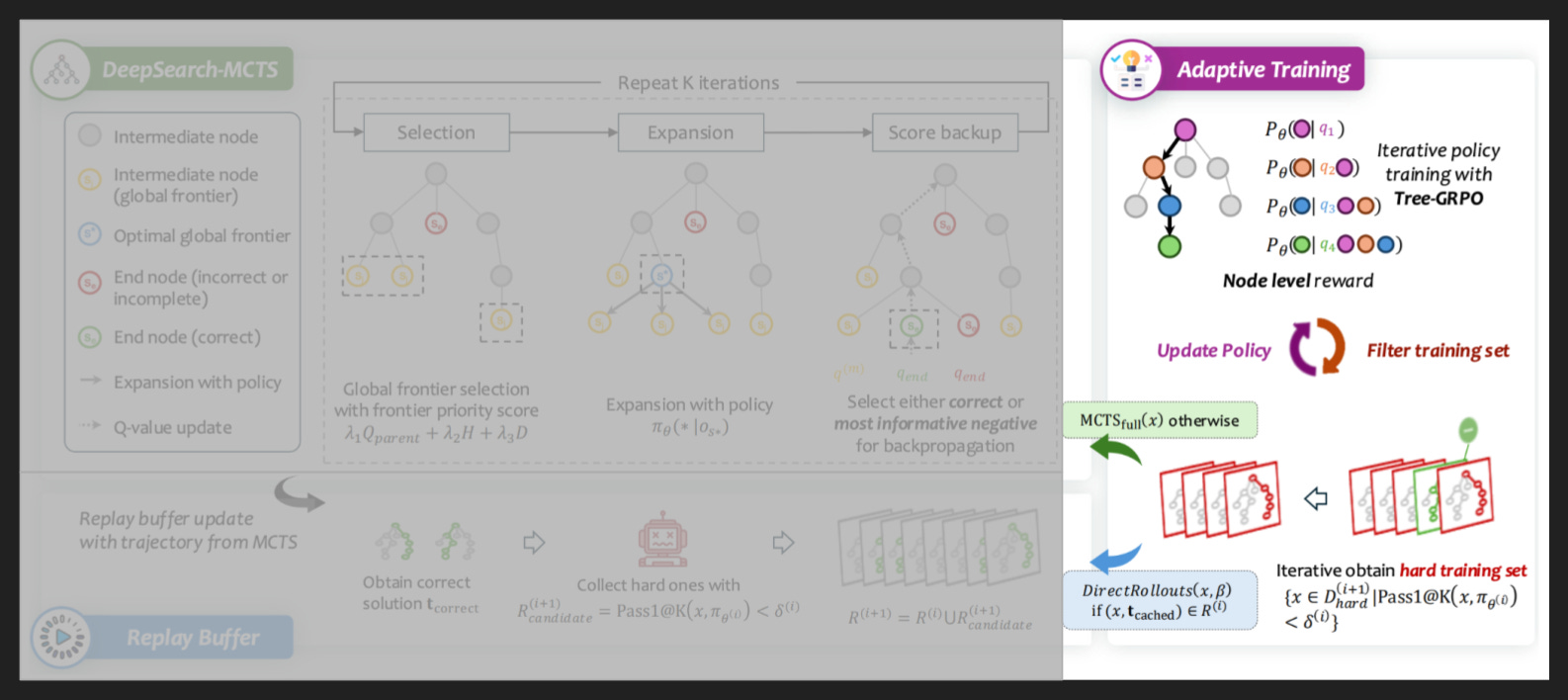
Then the last bit is how they train.
Basically they’re taking GRPO, which is an algorithm for turning rewards into model updates, and they’re adding rewards on the node level. Like in regular GRPO you just give one reward to the whole response, which is admittedly pretty imprecise; there might be a lot of text in the response that isn’t actually helpful. So to take advantage of this MCTS tree where we know which nodes were more or less helpful, this Tree-GRPO algorithm uses the q score at each node in the correct reasoning path as a reward and updates the model accordingly.
The bit at the bottom with the red and green tree drawings is about filtering your initial training set. We only need to do this whole MCTS process with problems where the model hasn’t gotten a correct reasoning path yet. For cases where the model is still bad at the problem, but has gotten it right at least once, you revert back to the normal RLVR thing of just passing in the problem and checking the final answer, what they call a “direct rollout”. And as we mentioned in the last slide, if a problem is too easy then we stop training on it altogether.
Now if you’ve been at Scale for a bit or have the relevant background, you might be thinking, isn’t this step-level reward thing pretty similar to process supervision? And even though the authors don’t make this comparison, I think you’d be right to.
For those unfamiliar, process supervision is when you have a human label each reasoning step as correct or incorrect. You then use that data to train a process reward model, a PRM, which you then use like any other reward model in your RL training loop.
So the two key differences are: one, process supervision directly assigns credit rather than calculating it based on correct paths and number of visits to a node; and two, process supervision is for training a PRM rather than directly training the generator. But the general idea of assigning more specific credit holds in both cases.
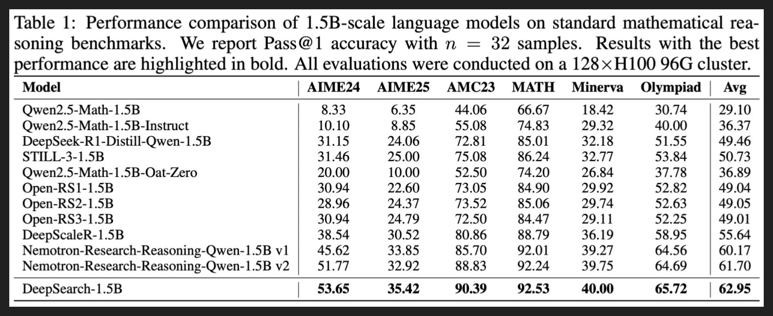
So this is where we net out. The starting point for DeepSearch was that Nemotron v2 one row above it in the table, and as you can see it’s not a big jump. Part of that is because there’s really not much room to move after a benchmark already hits 90%+ as with AMC23 and MATH, but even without those you’re looking at 0-3 points improvement. Real enough but not amazing.
And here I want to provide some other background and context, which I typically provide up front but I didn’t want to tip my hand here.
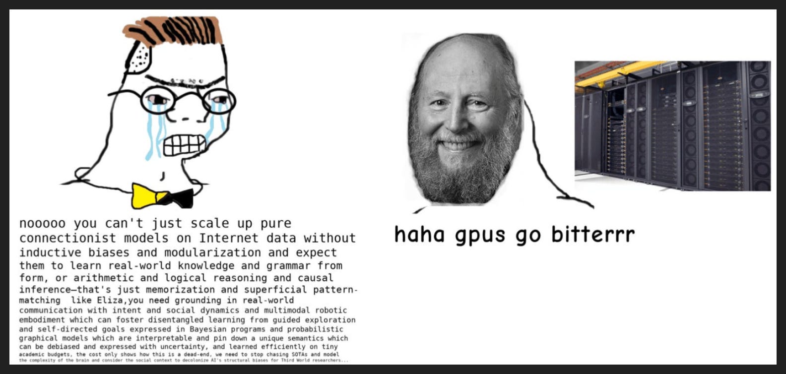
That bit of background is The Bitter Lesson.
In March of 2019 a famous computer scientist wrote a famous essay. That man was Rich Sutton, the father of reinforcement learning. That essay was The Bitter Lesson, describing the one constant he observed in his 35 years of work on AI.
I’m going to read the first paragraph verbatim:
“The biggest lesson that can be read from 70 years of AI research is that general methods that leverage computation are ultimately the most effective, and by a large margin. The ultimate reason for this is Moore's law, or rather its generalization of continued exponentially falling cost per unit of computation. Most AI research has been conducted as if the computation available to the agent were constant (in which case leveraging human knowledge would be one of the only ways to improve performance) but, over a slightly longer time than a typical research project, massively more computation inevitably becomes available. Seeking an improvement that makes a difference in the shorter term, researchers seek to leverage their human knowledge of the domain, but the only thing that matters in the long run is the leveraging of computation. These two need not run counter to each other, but in practice they tend to. Time spent on one is time not spent on the other. There are psychological commitments to investment in one approach or the other. And the human-knowledge approach tends to complicate methods in ways that make them less suited to taking advantage of general methods leveraging computation. There were many examples of AI researchers' belated learning of this bitter lesson, and it is instructive to review some of the most prominent.”
He mentions chess, Go, speech recognition, and computer vision as fields where attempting to program in human knowledge failed, while throwing more computation at searching and learning succeeded. Chess and Go are examples of search scaling up, with AI looking many moves ahead into many possible futures at the same time. Speech recognition and computer vision are examples of learning scaling up, with bigger neural networks, bigger datasets, and more compute.
He couldn’t have known this in 2019, but we can now add natural language to that list. Getting AIs to talk has a long history, and until relatively recently it involved programming our rules of grammar into the model. But LLMs don’t work like that. As the compute became available, we spent more on learning and gave up the human-derived rules, and now we have models that can write better than most people can.
So the question for our paper is, is Monte Carlo Tree Search bitter? Or are we programming in human methods for short-term gain, forgetting the opportunity cost of neglecting more bitter methods?
Certainly I think RLVR is more bitter. If all we do is reward models for getting right answers, we’re giving them complete freedom to be their own sorts of minds. If we enforce the paradigm of step-by-step thinking like in MCTS, even if MCTS is a method of searching and did work for mastering Go, I think we lose something.
In fact the DeepSeek R1 paper demonstrated it too. They trained two versions of their model: R1, which used a little SFT to teach a reasoning format and then RLVR to improve reasoning; and R1-Zero, which skipped the SFT and just did RLVR. R1-Zero ultimately did better BUT had some usability issues, like sometimes switching between English and Chinese. So we forced human strictures onto a machine mind and hurt performance as a result.
I’m not disputing the results of this paper - I believe MCTS did help performance - but I am skeptical that this amount of structure and method is what really breaks LLMs through to the next level.
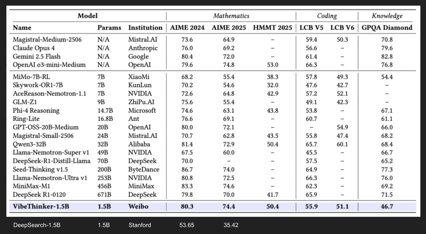
Now by sheer coincidence ANOTHER small reasoning finetune of Qwen2.5-1.5B came out while I was making this presentation. VibeThinker drops some crazy benchmark scores, rivaling fairly recent models 10-100x its size. Just for context on this model size, you could run a quantized version of this on your phone today. In fact, the newest Pixel phones ship with a 1.8B version of Gemini. 1.5B is also the size of GPT-2, which like The Bitter Lesson came out in 2019, although The Bitter Lesson came first.
Anyway we’re not going to review that paper, but I will note there are no specialized structures in their method; they do SFT then RL, with some tweaks to which SFT checkpoints they RL on and what problems to train on in RL, both of which are bitter in my view.
My Takeaways
MCTS seems great for games with discrete states, but I don’t buy it for languages (natural, math, code)
Maybe we will see MCTS for agent domains with discrete states
Computer use?
I do buy entropy as a guide for what you train on
I feel like we are due for another breakthrough
Incremental gains are still happening on track though (see Gemini 3) - “there is no wall”